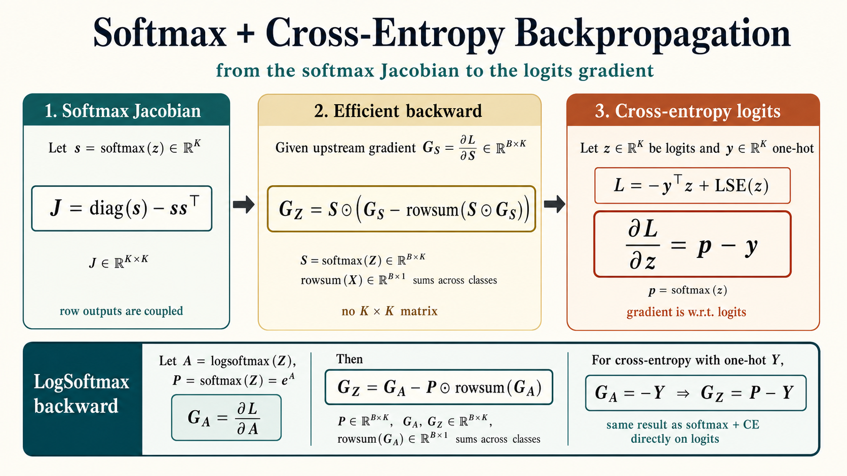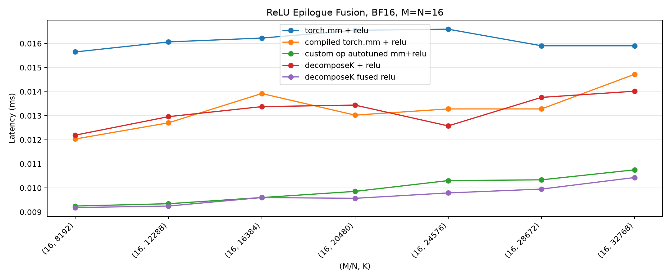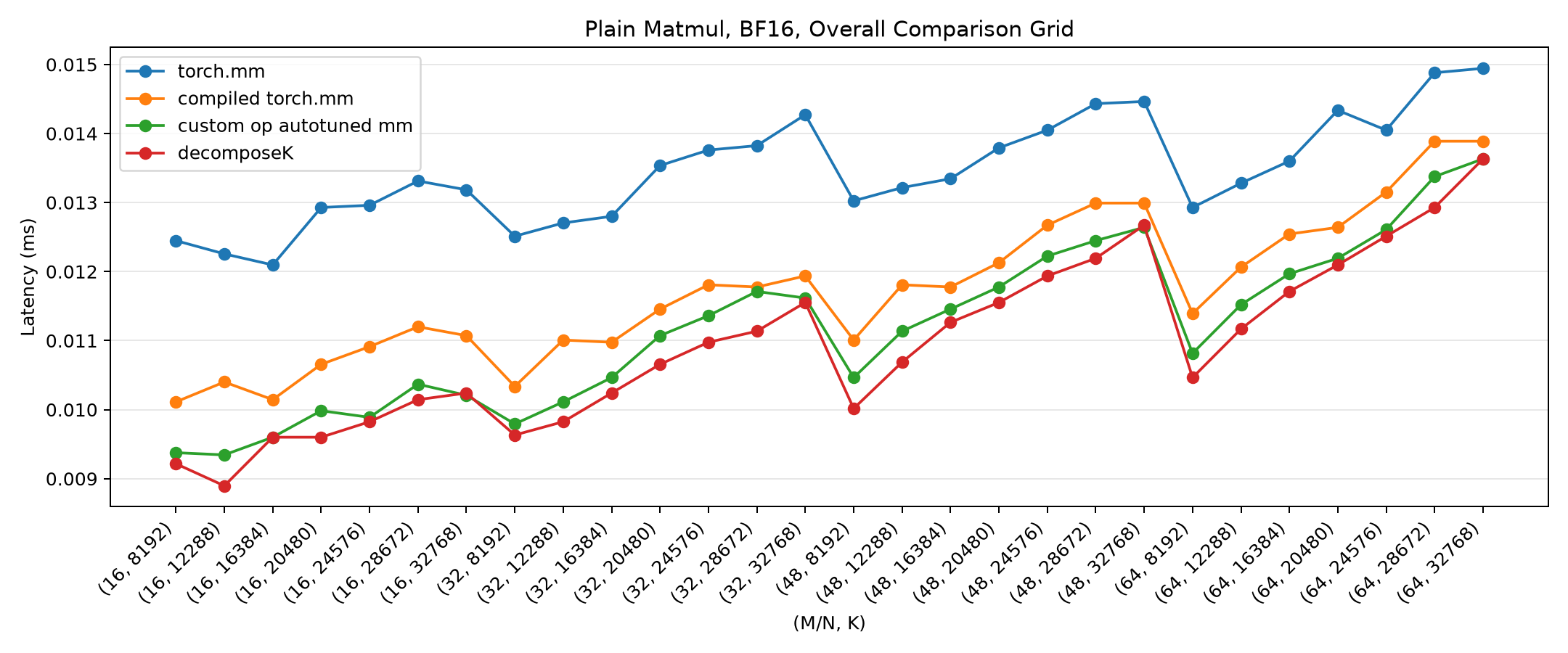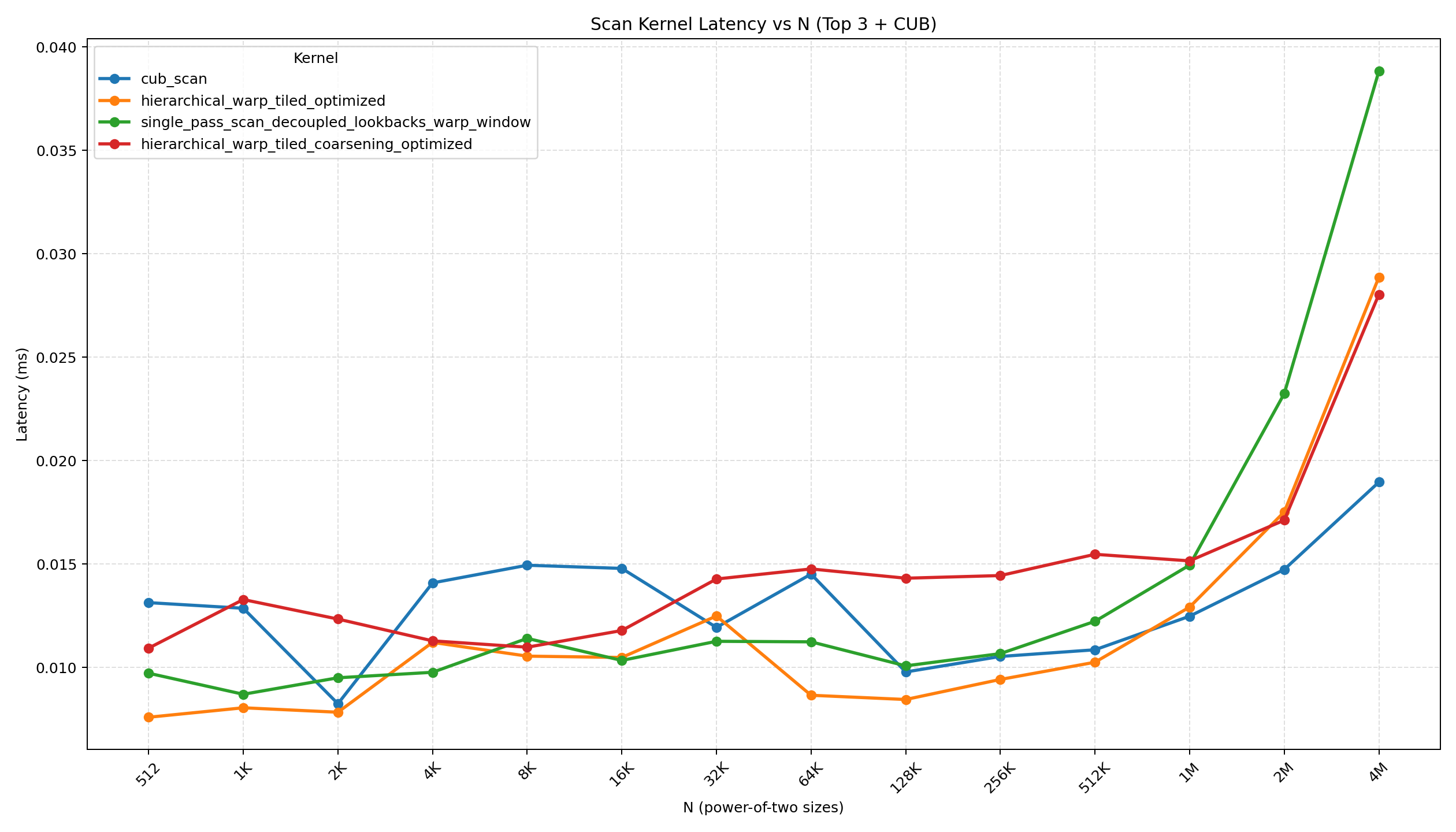
<?xml version="1.0" encoding="utf-8"?><feed xmlns="http://www.w3.org/2005/Atom" xml:lang="en"><generator uri="https://jekyllrb.com/" version="4.3.3">Jekyll</generator><link href="https://shreyansh26.github.io/feed.xml" rel="self" type="application/atom+xml"/><link href="https://shreyansh26.github.io/" rel="alternate" type="text/html" hreflang="en"/><updated>2026-07-06T19:49:33+00:00</updated><id>https://shreyansh26.github.io/feed.xml</id><title type="html">blank</title><subtitle>Shreyansh&apos;s personal website. </subtitle><entry><title type="html">Softmax and Cross-Entropy Backward Pass</title><link href="https://shreyansh26.github.io/post/2026-07-06_softmax-cross-entropy-backprop/" rel="alternate" type="text/html" title="Softmax and Cross-Entropy Backward Pass"/><published>2026-07-06T00:00:00+00:00</published><updated>2026-07-06T00:00:00+00:00</updated><id>https://shreyansh26.github.io/post/softmax-cross-entropy-backprop</id><content type="html" xml:base="https://shreyansh26.github.io/post/2026-07-06_softmax-cross-entropy-backprop/"><![CDATA[<div class="outer"> <figure class="image" style="width: 82%;"> <img src="/assets/img/posts_images/softmax_cross_entropy_backward/featured.png" alt="Softmax backward is a Jacobian-vector product. Cross-entropy with logits turns it into the familiar p - y gradient."/> <figcaption>Softmax backward is a Jacobian-vector product. Cross-entropy with logits turns it into the familiar p - y gradient.</figcaption> <br/> </figure> </div> <style>.outer{display:block;text-align:center;max-width:100%}.image{display:inline-block;max-width:100%;margin:0 auto}.image img{display:block;width:100%;height:auto;max-width:100%}figure.embed,figure.embed-top,figure.overlay,figure.embed-over{display:inline-block;text-align:initial;vertical-align:top;position:relative;margin:.5em;font-size:.8em;background:white;overflow:hidden}figure.embed img,figure.embed-top img,figure.overlay img,figure.embed-over img{display:block;margin-left:auto;margin-right:auto}figure.embed figcaption,figure.embed-top figcaption,figure.overlay figcaption,figure.embed-over figcaption{width:100%;padding:.5em;color:rgba(50,50,50,1);background:rgba(200,200,200,0.825)}figcaption{display:block;font-size:80%}</style> <p>Softmax plus cross-entropy gets summarized so often as <code class="language-plaintext highlighter-rouge">p - y</code> that it is easy to forget where that expression comes from:</p> \[\frac{\partial L}{\partial z} = p - y\] <p>The formula is right, but two implementation details are easy to miss.</p> <p>First, softmax is not elementwise. Every output probability depends on every logit in the same row because the classes share one normalization denominator. So the backward pass is a Jacobian-vector product, not a coordinate-wise derivative.</p> <p>Second, \(p-y\) is a gradient with respect to <strong>logits</strong>, not probabilities. It shows up only after the log in cross-entropy interacts with the softmax Jacobian.</p> <p>This note walks through both pieces: the general softmax backward pass for an arbitrary upstream gradient, and the cross-entropy/logsoftmax case that produces the expression used in training code.</p> <h2 id="setup">Setup</h2> <p>For one row, let the logits be</p> \[z \in \mathbb{R}^K\] <p>and define</p> \[s = \operatorname{softmax}(z), \qquad s_j = \frac{e^{z_j}}{\sum_{\ell=1}^{K} e^{z_\ell}}.\] <p>For a batch, write the logits as</p> \[Z \in \mathbb{R}^{B \times K}\] <p>and the softmax outputs as</p> \[S \in \mathbb{R}^{B \times K}.\] <p>Softmax is applied row-wise:</p> \[S_{ij} = \frac{e^{Z_{ij}}}{\sum_{\ell=1}^{K} e^{Z_{i\ell}}}.\] <p>Here \(i\) indexes the batch row. The indices \(j\) and \(k\) index classes, vocabulary entries, or whatever lives on the final axis. Rows do not interact, so it is enough to derive the formula for one row and apply it to the whole batch.</p> <h2 id="the-softmax-derivative">The Softmax Derivative</h2> <p>For one batch row \(i\), define the row-wise denominator</p> \[D_i = \sum_{\ell=1}^{K} e^{Z_{i\ell}}.\] <p>Then</p> \[S_{ij} = \frac{e^{Z_{ij}}}{D_i}.\] <p>We want the derivative</p> \[\frac{\partial S_{ij}}{\partial Z_{ik}},\] <p>This asks a local question: if we nudge the logit for class \(k\), what happens to the softmax probability assigned to class \(j\)?</p> <p>Using the quotient rule,</p> \[\frac{\partial S_{ij}}{\partial Z_{ik}} = \frac{ D_i \frac{\partial e^{Z_{ij}}}{\partial Z_{ik}} - e^{Z_{ij}} \frac{\partial D_i}{\partial Z_{ik}} }{ D_i^2 }.\] <p>The numerator derivative depends on whether \(j=k\):</p> \[\frac{\partial e^{Z_{ij}}}{\partial Z_{ik}} = e^{Z_{ij}}\delta_{jk},\] <p>where</p> \[\delta_{jk} = \begin{cases} 1, &amp; j=k, \\ 0, &amp; j \neq k. \end{cases}\] <p>The denominator derivative is</p> \[\frac{\partial D_i}{\partial Z_{ik}} = \frac{\partial}{\partial Z_{ik}} \sum_{\ell=1}^{K} e^{Z_{i\ell}} = e^{Z_{ik}}.\] <p>Substituting both pieces gives</p> \[\begin{aligned} \frac{\partial S_{ij}}{\partial Z_{ik}} &amp;= \frac{D_i e^{Z_{ij}}\delta_{jk} - e^{Z_{ij}}e^{Z_{ik}}}{D_i^2} \\ &amp;= \frac{e^{Z_{ij}}}{D_i}\delta_{jk} - \frac{e^{Z_{ij}}}{D_i}\frac{e^{Z_{ik}}}{D_i}. \end{aligned}\] <p>Since</p> \[\frac{e^{Z_{ij}}}{D_i}=S_{ij}, \qquad \frac{e^{Z_{ik}}}{D_i}=S_{ik},\] <p>we get the scalar softmax derivative:</p> \[\boxed{ \frac{\partial S_{ij}}{\partial Z_{ik}} = S_{ij}(\delta_{jk}-S_{ik}) }\] <p>This compact expression contains both cases:</p> \[\frac{\partial S_{ij}}{\partial Z_{ij}} = S_{ij}(1-S_{ij})\] <p>and, for \(j \neq k\),</p> \[\frac{\partial S_{ij}}{\partial Z_{ik}} = -S_{ij}S_{ik}.\] <p>The sign tells the story. Increasing a logit’s own value increases its own probability. Increasing some other logit gives that other class more of the shared denominator, so this probability goes down.</p> <h2 id="the-jacobian">The Jacobian</h2> <p>For a fixed row \(i\), collect all derivatives into a Jacobian matrix</p> \[J_i \in \mathbb{R}^{K \times K}, \qquad J_{i,jk} = \frac{\partial S_{ij}}{\partial Z_{ik}}.\] <p>The diagonal entries are \(S_{ij}(1-S_{ij})\). The off-diagonal entries are \(-S_{ij}S_{ik}\). In matrix form:</p> \[\boxed{ J_i = \operatorname{diag}(S_i) - S_i S_i^\top }\] <p>because</p> \[{\operatorname{diag}(S_i)}_{jk} = S_{ij}\delta_{jk}\] <p>and</p> \[{(S_iS_i^\top)}_{jk}=S_{ij}S_{ik}.\] <p>So each entry is</p> \[{(\operatorname{diag}(S_i)-S_iS_i^\top)}_{jk} = S_{ij}\delta_{jk}-S_{ij}S_{ik} = S_{ij}(\delta_{jk}-S_{ik}).\] <p>This Jacobian is dense, but it is also highly structured. We definitely do not want to materialize a \(K \times K\) matrix for every row. For a language model vocabulary, \(K\) can be tens or hundreds of thousands. The backward pass needs the Jacobian-vector product, not the Jacobian itself.</p> <p>There is a clean reason this Jacobian is symmetric. Define</p> \[\operatorname{LSE}(z) = \log \sum_{k=1}^{K} e^{z_k}.\] <p>Its gradient is softmax:</p> \[\nabla_z \operatorname{LSE}(z) = \operatorname{softmax}(z).\] <p>So the softmax Jacobian is the Hessian of logsumexp:</p> \[J_{\operatorname{softmax}}(z) = \nabla_z^2 \operatorname{LSE}(z).\] <p>For a smooth scalar function, the Hessian is symmetric. That is why \(J_i^\top=J_i\) in this case.</p> <h2 id="backpropagating-through-softmax">Backpropagating Through Softmax</h2> <p>Let the upstream gradient for one row be</p> \[G_{S_i} = \frac{\partial L}{\partial S_i}.\] <p>For a vector function \(y=f(x)\), the usual column-vector backpropagation rule is</p> \[g_x = J^\top g_y.\] <p>For softmax, \(J_i\) is symmetric, so</p> \[G_{Z_i} = J_i^\top G_{S_i} = J_iG_{S_i}.\] <p>Now expand the multiplication:</p> \[\begin{aligned} G_{Z_i} &amp;= \left(\operatorname{diag}(S_i)-S_iS_i^\top\right)G_{S_i} \\ &amp;= \operatorname{diag}(S_i)G_{S_i} - S_iS_i^\top G_{S_i}. \end{aligned}\] <p>The first term is elementwise multiplication:</p> \[\operatorname{diag}(S_i)G_{S_i} = S_i \odot G_{S_i}.\] <p>The second term has a scalar dot product inside:</p> \[S_iS_i^\top G_{S_i} = S_i(S_i^\top G_{S_i}).\] <p>Therefore,</p> \[G_{Z_i} = S_i \odot G_{S_i} - S_i(S_i^\top G_{S_i}).\] <p>Factoring out \(S_i\) coordinate-wise:</p> \[\boxed{ G_{Z_i} = S_i \odot \left(G_{S_i} - S_i^\top G_{S_i}\right) }\] <p>Elementwise:</p> \[\boxed{ G_{Z,ij} = S_{ij} \left( G_{S,ij} - \sum_{k=1}^{K} S_{ik}G_{S,ik} \right) }\] <p>This computes the same thing as the full Jacobian multiply, but the actual work is just a row-wise dot product and an elementwise multiply:</p> <div class="language-python highlighter-rouge"><div class="highlight"><pre class="highlight"><code><span class="k">def</span> <span class="nf">softmax_backward</span><span class="p">(</span><span class="n">grad_out</span><span class="p">,</span> <span class="n">softmax_out</span><span class="p">):</span>
    <span class="n">dot</span> <span class="o">=</span> <span class="p">(</span><span class="n">softmax_out</span> <span class="o">*</span> <span class="n">grad_out</span><span class="p">).</span><span class="nf">sum</span><span class="p">(</span><span class="n">dim</span><span class="o">=-</span><span class="mi">1</span><span class="p">,</span> <span class="n">keepdim</span><span class="o">=</span><span class="bp">True</span><span class="p">)</span>
    <span class="k">return</span> <span class="n">softmax_out</span> <span class="o">*</span> <span class="p">(</span><span class="n">grad_out</span> <span class="o">-</span> <span class="n">dot</span><span class="p">)</span>
</code></pre></div></div> <p>Here <code class="language-plaintext highlighter-rouge">grad_out</code> is \(\partial L / \partial S\), and <code class="language-plaintext highlighter-rouge">softmax_out</code> is the saved softmax output \(S\) from the forward pass. The <code class="language-plaintext highlighter-rouge">keepdim=True</code> keeps the dot product shaped as \(B \times 1\) so it broadcasts across the class dimension.</p> <p>As a quick sanity check, each row of \(G_Z\) sums to zero. That has to happen: adding the same constant to every logit in a row does not change softmax, so the backward pass should not push in that all-ones direction.</p> <h2 id="cross-entropy-with-logits">Cross-Entropy With Logits</h2> <p>Now let the target be \(y\). For a one-hot target, exactly one coordinate is \(1\). For label smoothing or soft targets, assume \(y\) is a normalized target distribution:</p> \[\sum_{j=1}^{K} y_j = 1.\] <p>The cross-entropy loss for one example is</p> \[L = -\sum_{j=1}^{K} y_j \log p_j,\] <p>where</p> \[p = \operatorname{softmax}(z).\] <p>Since</p> \[\log p_j = \log \left(\frac{e^{z_j}}{\sum_{k=1}^{K} e^{z_k}}\right) = z_j - \log \sum_{k=1}^{K} e^{z_k},\] <p>we can rewrite the loss directly as a function of logits:</p> \[\begin{aligned} L &amp;= -\sum_{j=1}^{K} y_j \left( z_j - \log \sum_{k=1}^{K} e^{z_k} \right) \\ &amp;= -\sum_{j=1}^{K} y_jz_j + \left(\sum_{j=1}^{K} y_j\right) \log \sum_{k=1}^{K} e^{z_k}. \end{aligned}\] <p>Because \(\sum_j y_j=1\),</p> \[\boxed{ L = -y^\top z + \operatorname{LSE}(z) }\] <p>Differentiate with respect to logit \(z_i\):</p> \[\frac{\partial}{\partial z_i}(-y^\top z) = -y_i\] <p>and</p> \[\frac{\partial}{\partial z_i}\operatorname{LSE}(z) = \frac{e^{z_i}}{\sum_{k=1}^{K}e^{z_k}} = p_i.\] <p>Therefore,</p> \[\boxed{ \frac{\partial L}{\partial z_i} = p_i-y_i }\] <p>and in vector form,</p> \[\boxed{ \frac{\partial L}{\partial z} = p-y }\] <p>For the target class \(t\), this is</p> \[\frac{\partial L}{\partial z_t} = p_t-1.\] <p>For a non-target class \(i \neq t\), it is</p> \[\frac{\partial L}{\partial z_i} = p_i.\] <p>In code, the plain batch-mean version looks like this:</p> <div class="language-python highlighter-rouge"><div class="highlight"><pre class="highlight"><code><span class="n">probs</span> <span class="o">=</span> <span class="n">torch</span><span class="p">.</span><span class="nf">softmax</span><span class="p">(</span><span class="n">logits</span><span class="p">,</span> <span class="n">dim</span><span class="o">=-</span><span class="mi">1</span><span class="p">)</span>
<span class="n">B</span> <span class="o">=</span> <span class="n">logits</span><span class="p">.</span><span class="n">shape</span><span class="p">[</span><span class="mi">0</span><span class="p">]</span>
<span class="n">dlogits</span> <span class="o">=</span> <span class="n">probs</span><span class="p">.</span><span class="nf">clone</span><span class="p">()</span>
<span class="n">dlogits</span><span class="p">[</span><span class="n">torch</span><span class="p">.</span><span class="nf">arange</span><span class="p">(</span><span class="n">B</span><span class="p">,</span> <span class="n">device</span><span class="o">=</span><span class="n">logits</span><span class="p">.</span><span class="n">device</span><span class="p">),</span> <span class="n">targets</span><span class="p">]</span> <span class="o">-=</span> <span class="mi">1</span>
<span class="n">dlogits</span> <span class="o">/=</span> <span class="n">B</span>
</code></pre></div></div> <p>The final <code class="language-plaintext highlighter-rouge">dlogits</code> tensor is not a probability distribution. It is the gradient \(\partial L/\partial Z\). For a batch mean reduction with no class weights and no ignored labels,</p> \[\boxed{ \frac{\partial L_{\text{batch}}}{\partial Z} = \frac{1}{B}(P-Y) }\] <h2 id="the-same-result-through-the-softmax-jacobian">The Same Result Through the Softmax Jacobian</h2> <p>The logsumexp derivation is the shortest route. It is still useful to check the same result by chaining cross-entropy through the softmax Jacobian.</p> <p>Starting from</p> \[L = -\sum_{i=1}^{K} y_i \log p_i,\] <p>the gradient with respect to probabilities is</p> \[g_p = \frac{\partial L}{\partial p} = -\frac{y}{p}\] <p>elementwise.</p> <p>The softmax backward formula from above is</p> \[g_z = p \odot \left(g_p - p^\top g_p\right).\] <p>Compute the scalar dot product:</p> \[p^\top g_p = \sum_{i=1}^{K} p_i\left(-\frac{y_i}{p_i}\right) = -\sum_{i=1}^{K} y_i = -1.\] <p>Then</p> \[\begin{aligned} g_z &amp;= p \odot \left(-\frac{y}{p} + 1\right) \\ &amp;= -y+p \\ &amp;= \boxed{p-y}. \end{aligned}\] <p>This is the cancellation people usually have in mind. The dense softmax Jacobian is still there mathematically, but the \(1/p_i\) term from differentiating the log collapses it into a simple logits gradient.</p> <h2 id="logsoftmax-backward">LogSoftmax Backward</h2> <p>In practice, frameworks usually avoid computing softmax probabilities and then taking a log. They use logsoftmax or a fused cross-entropy kernel, because logsumexp can be computed stably by subtracting the row maximum before exponentiating.</p> <p>Define</p> \[a = \operatorname{logsoftmax}(z), \qquad a_j = \log p_j = z_j-\operatorname{LSE}(z).\] <p>Differentiate:</p> \[\frac{\partial a_j}{\partial z_i} = \delta_{ji} - \frac{\partial \operatorname{LSE}(z)}{\partial z_i} = \delta_{ji}-p_i.\] <p>Let</p> \[g_a = \frac{\partial L}{\partial a}.\] <p>Then</p> \[\begin{aligned} g_{z_i} &amp;= \sum_{j=1}^{K} g_{a_j} \frac{\partial a_j}{\partial z_i} \\ &amp;= \sum_{j=1}^{K} g_{a_j}(\delta_{ji}-p_i) \\ &amp;= g_{a_i} - p_i\sum_{j=1}^{K}g_{a_j}. \end{aligned}\] <p>So the vector form is</p> \[\boxed{ g_z = g_a - p(\mathbf{1}^\top g_a) }\] <p>and the batch form is</p> \[\boxed{ G_Z = G_A - P \odot \operatorname{rowsum}(G_A) }\] <p>Here <code class="language-plaintext highlighter-rouge">rowsum</code> has shape \(B \times 1\) and broadcasts across the final axis.</p> <p>In code:</p> <div class="language-python highlighter-rouge"><div class="highlight"><pre class="highlight"><code><span class="k">def</span> <span class="nf">logsoftmax_backward</span><span class="p">(</span><span class="n">grad_out</span><span class="p">,</span> <span class="n">softmax_out</span><span class="p">):</span>
    <span class="n">rowsum</span> <span class="o">=</span> <span class="n">grad_out</span><span class="p">.</span><span class="nf">sum</span><span class="p">(</span><span class="n">dim</span><span class="o">=-</span><span class="mi">1</span><span class="p">,</span> <span class="n">keepdim</span><span class="o">=</span><span class="bp">True</span><span class="p">)</span>
    <span class="k">return</span> <span class="n">grad_out</span> <span class="o">-</span> <span class="n">softmax_out</span> <span class="o">*</span> <span class="n">rowsum</span>
</code></pre></div></div> <p>For negative log-likelihood or cross-entropy,</p> \[L = -\sum_{j=1}^{K}y_ja_j,\] <p>so</p> \[g_a = -y.\] <p>Because</p> \[\mathbf{1}^\top g_a = -\sum_j y_j = -1,\] <p>substituting into the logsoftmax backward pass gives</p> \[g_z = -y - p(-1) = p-y.\] <p>At that point, all three routes agree:</p> \[\boxed{ \text{cross-entropy with softmax logits backward} = \frac{\partial L}{\partial z} = \operatorname{softmax}(z)-y }\] <p>and, for a plain batch mean,</p> \[\boxed{ \frac{\partial L}{\partial Z} = \frac{1}{B}(P-Y). }\] <h2 id="a-small-numerical-check">A Small Numerical Check</h2> <p>Suppose the predicted probabilities and one-hot target are</p> \[p = [0.659,\;0.242,\;0.099], \qquad y = [1,\;0,\;0].\] <p>Then</p> \[\frac{\partial L}{\partial z} = p-y = [-0.341,\;0.242,\;0.099].\] <p>The target-class gradient is negative. Under gradient descent,</p> \[z \leftarrow z - \eta \nabla_z L,\] <p>subtracting a negative value increases the target logit. The non-target gradients are positive, so their logits decrease. That matches the training signal we expected.</p> <h2 id="what-to-remember">What to Remember</h2> <p>Softmax backward is a structured Jacobian-vector product:</p> \[\boxed{ G_Z = S \odot \left(G_S - \operatorname{rowsum}(S \odot G_S)\right) }\] <p>Cross-entropy with logits simplifies to:</p> \[\boxed{ G_Z = P - Y }\] <p>with whatever scaling the loss reduction adds.</p> <p>The mental model I use is this: softmax couples the classes through a shared denominator, and cross-entropy contributes the reciprocal probability term that removes that coupling in the logits gradient. That is why the training code can use a simple \(P-Y\) update even though softmax itself has a dense Jacobian.</p> <hr/> <p> </p> <script type="text/javascript" src="//downloads.mailchimp.com/js/signup-forms/popup/unique-methods/embed.js" data-dojo-config="usePlainJson: true, isDebug: false"></script> <div class="button_cont" align="center"><button id="openpopup" class="example_a">Subscribe to my posts!</button></div> <style>.example_a{color:#fff!important;text-transform:uppercase;text-decoration:none;background:#3f51b5;padding:20px;border-radius:5px;cursor:pointer;display:inline-block;border:0;transition:all .4s ease 0}.example_a:hover{background:#434343;letter-spacing:1px;-webkit-box-shadow:0 5px 40px -10px rgba(0,0,0,0.57);-moz-box-shadow:0 5px 40px -10px rgba(0,0,0,0.57);box-shadow:5px 40px -10px rgba(0,0,0,0.57);transition:all .4s ease 0}</style> <script type="text/javascript">function showMailingPopUp(){window.dojoRequire(["mojo/signup-forms/Loader"],function(o){o.start({baseUrl:"mc.us4.list-manage.com",uuid:"0b10ac14f50d7f4e7d11cf26a",lid:"667a1bb3da",uniqueMethods:!0})}),document.cookie="MCPopupClosed=;path=/;expires=Thu, 01 Jan 1970 00:00:00 UTC"}document.getElementById("openpopup").onclick=function(){showMailingPopUp()};</script> <p> </p> <script data-name="BMC-Widget" data-cfasync="false" src="https://cdnjs.buymeacoffee.com/1.0.0/widget.prod.min.js" data-id="shreyanshsingh" data-description="Support me on Buy me a coffee!" data-message="" data-color="#FF5F5F" data-position="Right" data-x_margin="18" data-y_margin="18"></script> <p>Follow me on <a href="https://twitter.com/shreyansh_26">Twitter</a>, <a href="https://github.com/shreyansh26">Github</a> or connect on <a href="https://www.linkedin.com/in/shreyansh26/">LinkedIn</a>.</p>]]></content><author><name>Shreyansh Singh</name></author><category term="ML"/><category term="ml"/><category term="math"/><summary type="html"><![CDATA[A step-by-step derivation of softmax, logsoftmax, and cross-entropy backward passes: how the softmax Jacobian turns into a row-wise dot product, and why the logits gradient is p - y.]]></summary></entry><entry><title type="html">Decompose-K: From torch.compile to Hand-Tuned Triton Kernels for Skinny Large‑K Matmuls</title><link href="https://shreyansh26.github.io/post/2026-06-21_decompose-k-triton/" rel="alternate" type="text/html" title="Decompose-K: From torch.compile to Hand-Tuned Triton Kernels for Skinny Large‑K Matmuls"/><published>2026-06-21T00:00:00+00:00</published><updated>2026-06-21T00:00:00+00:00</updated><id>https://shreyansh26.github.io/post/decompose-k-triton</id><content type="html" xml:base="https://shreyansh26.github.io/post/2026-06-21_decompose-k-triton/"><![CDATA[<p><em>The source code for this post is available on GitHub: <a href="https://github.com/shreyansh26/MLSys-Experiments/tree/main/decompose-k">shreyansh26/MLSys-Experiments/decompose-k</a>.</em></p> <p><em>The idea of Decompose-K and the custom-op autotuning workflow comes from the PyTorch Conference talk <a href="https://www.youtube.com/watch?v=rKQbHSs7dBo">Lightning Talk: Faster Than SOTA Kernels in Torch.compile With Subgraph Fusions and Custom Op Autotuning - Elias Ellison &amp; Paul Zhang, Meta</a>. This post is my own implementation walkthrough and benchmark study built around that idea.</em></p> <hr/> <h2 id="the-skinny-large-k-matmul-problem">The skinny large-K matmul problem</h2> <p>A standard matmul is</p> <div class="language-text highlighter-rouge"><div class="highlight"><pre class="highlight"><code>C[M, N] = A[M, K] @ B[K, N]
</code></pre></div></div> <p>and the way a GPU GEMM extracts parallelism is by tiling the <code class="language-plaintext highlighter-rouge">M x N</code> output. Each program owns a <code class="language-plaintext highlighter-rouge">BLOCK_M x BLOCK_N</code> tile of <code class="language-plaintext highlighter-rouge">C</code> and streams over <code class="language-plaintext highlighter-rouge">K</code> to accumulate it. That works well when <code class="language-plaintext highlighter-rouge">M</code> and <code class="language-plaintext highlighter-rouge">N</code> are large, because there are many output tiles and the GPU has plenty of independent work to fill its streaming multiprocessors (SMs).</p> <p>The problem case is a <strong>skinny, K-dominant</strong> matmul: <code class="language-plaintext highlighter-rouge">M</code> and <code class="language-plaintext highlighter-rouge">N</code> are tiny while <code class="language-plaintext highlighter-rouge">K</code> is huge. Think <code class="language-plaintext highlighter-rouge">M = N = 16</code> with <code class="language-plaintext highlighter-rouge">K = 32768</code>, or a decode-time MoE router GEMM like <code class="language-plaintext highlighter-rouge">[T, 7168] @ [7168, 256]</code> where <code class="language-plaintext highlighter-rouge">T</code> can be as small as 1. Now the output is <code class="language-plaintext highlighter-rouge">16 x 16 = 256</code> elements, which is one or two tiles. The GPU has 132 SMs sitting idle while one or two programs serially walk a reduction of length 32768. The matmul is reduction-bound, but the standard tiling exposes almost no parallelism along the only large axis.</p> <p>Decompose-K is a restructuring that fixes exactly this mismatch. The basic idea is simple: if the only big dimension is <code class="language-plaintext highlighter-rouge">K</code>, then split <code class="language-plaintext highlighter-rouge">K</code> and parallelize over the split.</p> <h2 id="what-decompose-k-does">What Decompose-K does</h2> <div class="outer"> <figure class="image"> <img src="/assets/img/posts_images/decompose_k/decompose_k_cover.png" alt="Decompose-K splits the long K dimension into S chunks, runs the S partial GEMMs as a batched matmul, and sums the partials (with an optional fused epilogue on the reduction store)."/> <figcaption>Decompose-K splits the long K dimension into S chunks, runs the S partial GEMMs as a batched matmul, and sums the partials (with an optional fused epilogue on the reduction store).</figcaption> <br/> </figure> </div> <style>.outer{display:block;text-align:center;max-width:100%}.image{display:inline-block;max-width:100%;margin:0 auto}.image img{display:block;width:100%;height:auto;max-width:100%}figure.embed,figure.embed-top,figure.overlay,figure.embed-over{display:inline-block;text-align:initial;vertical-align:top;position:relative;margin:.5em;font-size:.8em;background:white;overflow:hidden}figure.embed img,figure.embed-top img,figure.overlay img,figure.embed-over img{display:block;margin-left:auto;margin-right:auto}figure.embed figcaption,figure.embed-top figcaption,figure.overlay figcaption,figure.embed-over figcaption{width:100%;padding:.5em;color:rgba(50,50,50,1);background:rgba(200,200,200,0.825)}figcaption{display:block;font-size:80%}</style> <p>Split the <code class="language-plaintext highlighter-rouge">K</code> dimension into <code class="language-plaintext highlighter-rouge">S</code> independent chunks, compute <code class="language-plaintext highlighter-rouge">S</code> partial GEMMs, then sum the partials:</p> <div class="language-text highlighter-rouge"><div class="highlight"><pre class="highlight"><code>A[M, K] @ B[K, N]
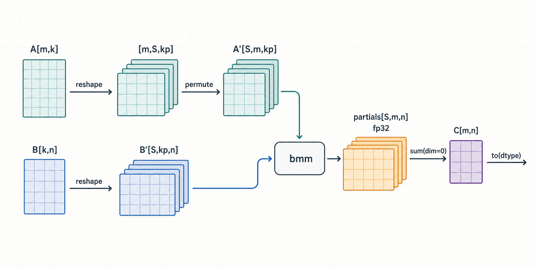
  -&gt; partials[S, M, N]
  -&gt; sum(partials, dim=0)
</code></pre></div></div> <p>Each partial is a smaller matmul over <code class="language-plaintext highlighter-rouge">K/S</code> of the reduction. The <code class="language-plaintext highlighter-rouge">S</code> partials are independent, so they become a batched matmul (<code class="language-plaintext highlighter-rouge">bmm</code>) with batch dimension <code class="language-plaintext highlighter-rouge">S</code>. The minimal PyTorch version makes this concrete:</p> <div class="language-python highlighter-rouge"><div class="highlight"><pre class="highlight"><code><span class="k">def</span> <span class="nf">decomposeK</span><span class="p">(</span><span class="n">a</span><span class="p">,</span> <span class="n">b</span><span class="p">,</span> <span class="n">k_splits</span><span class="p">):</span>
    <span class="n">m</span><span class="p">,</span> <span class="n">k</span> <span class="o">=</span> <span class="n">a</span><span class="p">.</span><span class="n">shape</span>
    <span class="n">n</span> <span class="o">=</span> <span class="n">b</span><span class="p">.</span><span class="n">shape</span><span class="p">[</span><span class="mi">1</span><span class="p">]</span>
    <span class="k">assert</span> <span class="n">k</span> <span class="o">%</span> <span class="n">k_splits</span> <span class="o">==</span> <span class="mi">0</span><span class="p">,</span> <span class="sh">"</span><span class="s">k must be divisible by k_splits</span><span class="sh">"</span>
    <span class="n">k_parts</span> <span class="o">=</span> <span class="n">k</span> <span class="o">//</span> <span class="n">k_splits</span>

    <span class="c1"># [m, k] -&gt; [m, k_splits, k_parts] -&gt; [k_splits, m, k_parts]
</span>    <span class="n">a_reshaped</span> <span class="o">=</span> <span class="n">a</span><span class="p">.</span><span class="nf">reshape</span><span class="p">(</span><span class="n">m</span><span class="p">,</span> <span class="n">k_splits</span><span class="p">,</span> <span class="n">k_parts</span><span class="p">).</span><span class="nf">permute</span><span class="p">(</span><span class="mi">1</span><span class="p">,</span> <span class="mi">0</span><span class="p">,</span> <span class="mi">2</span><span class="p">)</span>
    <span class="n">b_reshaped</span> <span class="o">=</span> <span class="n">b</span><span class="p">.</span><span class="nf">reshape</span><span class="p">(</span><span class="n">k_splits</span><span class="p">,</span> <span class="n">k_parts</span><span class="p">,</span> <span class="n">n</span><span class="p">)</span>        <span class="c1"># [k_splits, k_parts, n]
</span>
    <span class="n">result</span> <span class="o">=</span> <span class="n">torch</span><span class="p">.</span><span class="nf">bmm</span><span class="p">(</span><span class="n">a_reshaped</span><span class="p">,</span> <span class="n">b_reshaped</span><span class="p">,</span> <span class="n">out_dtype</span><span class="o">=</span><span class="n">torch</span><span class="p">.</span><span class="n">float32</span><span class="p">)</span>
    <span class="n">reduced_result</span> <span class="o">=</span> <span class="n">result</span><span class="p">.</span><span class="nf">sum</span><span class="p">(</span><span class="n">dim</span><span class="o">=</span><span class="mi">0</span><span class="p">)</span>
    <span class="k">return</span> <span class="n">reduced_result</span><span class="p">.</span><span class="nf">to</span><span class="p">(</span><span class="n">a</span><span class="p">.</span><span class="n">dtype</span><span class="p">)</span>
</code></pre></div></div> <p>The important part is what the reshape buys. For <code class="language-plaintext highlighter-rouge">M = N = 16</code>, <code class="language-plaintext highlighter-rouge">K = 32768</code>, <code class="language-plaintext highlighter-rouge">S = 64</code>:</p> <ul> <li><code class="language-plaintext highlighter-rouge">a_reshaped</code> is <code class="language-plaintext highlighter-rouge">[64, 16, 512]</code>, <code class="language-plaintext highlighter-rouge">b_reshaped</code> is <code class="language-plaintext highlighter-rouge">[64, 512, 16]</code>.</li> <li>The <code class="language-plaintext highlighter-rouge">bmm</code> now has 64 independent matmuls instead of one. That is 64 units of work the scheduler can spread across SMs, versus a single output tile before.</li> <li>Each partial accumulates only <code class="language-plaintext highlighter-rouge">512</code> of the reduction, not <code class="language-plaintext highlighter-rouge">32768</code>.</li> </ul> <p>We have traded one long serial reduction for <code class="language-plaintext highlighter-rouge">S</code> short parallel ones, plus a final reduction of the <code class="language-plaintext highlighter-rouge">S</code> partials. The partials are accumulated in fp32 (<code class="language-plaintext highlighter-rouge">out_dtype=torch.float32</code>) so the split does not cost accuracy relative to a single fp32-accumulated matmul.</p> <p>This is essentially <strong>split-K</strong>, but expressed at the tensor level as a <code class="language-plaintext highlighter-rouge">bmm</code> plus a reduction rather than as atomic adds into a single output tile. That distinction matters once we add an epilogue, which is the next point.</p> <h3 id="why-it-is-epilogue-friendly">Why it is epilogue-friendly</h3> <p>A split-K design that uses atomic adds into the output has a problem if you want to fuse an elementwise epilogue like ReLU: the output tile is not final until <em>every</em> split has finished its atomic contribution, so you cannot apply ReLU during the accumulation. You would need a separate pass after all atomics settle.</p> <p>Decompose-K keeps the partials in a separate <code class="language-plaintext highlighter-rouge">[S, M, N]</code> buffer and does an <strong>explicit</strong> reduction. That means the reduction step is the natural and only place where each output element becomes final, so an epilogue can be folded directly into the reduction’s store:</p> <div class="language-text highlighter-rouge"><div class="highlight"><pre class="highlight"><code>acc = sum over splits of partials[:, m, n]
acc = relu(acc)          # fused into the same kernel
store C[m, n] = acc
</code></pre></div></div> <p>No extra pointwise pass over <code class="language-plaintext highlighter-rouge">C</code>, no second read/write of the output. For tiny outputs that are memory-bound on the epilogue, this is a real saving, and we will measure it later (~1.2x–1.4x over an unfused ReLU).</p> <h3 id="where-it-is-worth-it">Where it is worth it</h3> <p>Decompose-K is attractive when:</p> <ul> <li><code class="language-plaintext highlighter-rouge">K</code> is very large and <code class="language-plaintext highlighter-rouge">M</code>/<code class="language-plaintext highlighter-rouge">N</code> are small (e.g. <code class="language-plaintext highlighter-rouge">M = N = 16..64</code>, <code class="language-plaintext highlighter-rouge">K = 8192..32768</code>).</li> <li>The workload is latency-sensitive and a single fixed shape matters more than a general GEMM. A concrete example is a <strong>DeepSeek-V3 MoE router GEMM</strong> <code class="language-plaintext highlighter-rouge">[T, 7168] @ [7168, 256]</code>, where decode has tiny dynamic <code class="language-plaintext highlighter-rouge">T = 1..256</code> and prefill has larger <code class="language-plaintext highlighter-rouge">T</code>.</li> <li>A fused epilogue like ReLU can ride along on the reduction.</li> </ul> <p>It is <em>not</em> worth it when <code class="language-plaintext highlighter-rouge">M</code> and <code class="language-plaintext highlighter-rouge">N</code> are already large enough to fill the GPU, when <code class="language-plaintext highlighter-rouge">K</code> is small, when <code class="language-plaintext highlighter-rouge">K</code> divides poorly for the candidate split counts, or when the extra <code class="language-plaintext highlighter-rouge">[S, M, N]</code> buffer and its reduction dominate the cost.</p> <p>The rest of this post is a tour of implementations of this one idea, from the laziest (<code class="language-plaintext highlighter-rouge">torch.compile</code>) to a hand-written Triton kernel that beats Inductor’s own autotuned choice. Every benchmark below is BF16 on an H100 (132 SMs), over the grid <code class="language-plaintext highlighter-rouge">M = N ∈ {16, 32, 48, 64}</code> and <code class="language-plaintext highlighter-rouge">K ∈ {8192, …, 32768}</code>.</p> <h2 id="baseline-just-call-torchcompile">Baseline: just call <code class="language-plaintext highlighter-rouge">torch.compile</code></h2> <p>The first thing to try is to write <code class="language-plaintext highlighter-rouge">decomposeK</code> in plain PyTorch and let Inductor handle the rest. The relevant detail is the compile mode. Across the three benchmark suites used throughout this post - a BF16 matmul with a fused ReLU epilogue (<code class="language-plaintext highlighter-rouge">epilogue-bf16</code>), a plain BF16 matmul (<code class="language-plaintext highlighter-rouge">matmul-bf16</code>), and a plain FP32 matmul - <code class="language-plaintext highlighter-rouge">max-autotune-no-cudagraphs</code> was the best mode, edging out <code class="language-plaintext highlighter-rouge">max-autotune</code>:</p> <div class="language-python highlighter-rouge"><div class="highlight"><pre class="highlight"><code><span class="n">decomposeK_compiled</span> <span class="o">=</span> <span class="n">torch</span><span class="p">.</span><span class="nf">compile</span><span class="p">(</span><span class="n">decomposeK</span><span class="p">,</span> <span class="n">mode</span><span class="o">=</span><span class="sh">"</span><span class="s">max-autotune-no-cudagraphs</span><span class="sh">"</span><span class="p">)</span>
</code></pre></div></div> <p><code class="language-plaintext highlighter-rouge">max-autotune</code> turns on Inductor’s template autotuning (it benchmarks several generated kernels and picks the fastest). The <code class="language-plaintext highlighter-rouge">-no-cudagraphs</code> variant skips CUDA graph capture, which for these tiny single-shot calls avoids capture overhead without losing the autotuning benefit.</p> <h3 id="what-does-naive-compilation-actually-emit">What does naive compilation actually emit?</h3> <p>Compiling the <code class="language-plaintext highlighter-rouge">decomposeK</code> function above (for the router shape <code class="language-plaintext highlighter-rouge">[64, 7168] @ [7168, 256]</code>, <code class="language-plaintext highlighter-rouge">S = 4</code>) produces two operations, which you can read off the Inductor output code:</p> <div class="language-python highlighter-rouge"><div class="highlight"><pre class="highlight"><code><span class="c1"># extern bmm into an fp32 partials buffer
</span><span class="n">buf0</span> <span class="o">=</span> <span class="nf">empty_strided_cuda</span><span class="p">((</span><span class="mi">4</span><span class="p">,</span> <span class="mi">64</span><span class="p">,</span> <span class="mi">256</span><span class="p">),</span> <span class="p">(</span><span class="mi">16384</span><span class="p">,</span> <span class="mi">256</span><span class="p">,</span> <span class="mi">1</span><span class="p">),</span> <span class="n">torch</span><span class="p">.</span><span class="n">float32</span><span class="p">)</span>
<span class="n">extern_kernels</span><span class="p">.</span><span class="nf">bmm_dtype</span><span class="p">(</span>
    <span class="nf">reinterpret_tensor</span><span class="p">(</span><span class="n">arg0_1</span><span class="p">,</span> <span class="p">(</span><span class="mi">4</span><span class="p">,</span> <span class="mi">64</span><span class="p">,</span> <span class="mi">1792</span><span class="p">),</span> <span class="p">...),</span>
    <span class="nf">reinterpret_tensor</span><span class="p">(</span><span class="n">arg1_1</span><span class="p">,</span> <span class="p">(</span><span class="mi">4</span><span class="p">,</span> <span class="mi">1792</span><span class="p">,</span> <span class="mi">256</span><span class="p">),</span> <span class="p">...),</span>
    <span class="n">out_dtype</span><span class="o">=</span><span class="n">torch</span><span class="p">.</span><span class="n">float32</span><span class="p">,</span> <span class="n">out</span><span class="o">=</span><span class="n">buf0</span><span class="p">)</span>

<span class="c1"># one generated pointwise kernel: sum over the 4 splits + cast to bf16
</span><span class="n">triton_poi_fused__to_copy_sum_0</span><span class="p">.</span><span class="nf">run</span><span class="p">(</span><span class="n">buf0</span><span class="p">,</span> <span class="n">buf1</span><span class="p">,</span> <span class="mi">16384</span><span class="p">,</span> <span class="p">...)</span>
</code></pre></div></div> <p>So the <code class="language-plaintext highlighter-rouge">bmm</code> goes to an external (cuBLAS) batched kernel, and the <code class="language-plaintext highlighter-rouge">sum(dim=0)</code> plus the <code class="language-plaintext highlighter-rouge">.to(bf16)</code> cast get fused into a single generated Triton pointwise kernel. The generated reduction kernel is literally an unrolled add of the <code class="language-plaintext highlighter-rouge">S = 4</code> slices:</p> <div class="language-python highlighter-rouge"><div class="highlight"><pre class="highlight"><code><span class="n">tmp0</span> <span class="o">=</span> <span class="n">tl</span><span class="p">.</span><span class="nf">load</span><span class="p">(</span><span class="n">in_ptr0</span> <span class="o">+</span> <span class="p">(</span><span class="n">x0</span><span class="p">),</span> <span class="bp">None</span><span class="p">)</span>
<span class="n">tmp1</span> <span class="o">=</span> <span class="n">tl</span><span class="p">.</span><span class="nf">load</span><span class="p">(</span><span class="n">in_ptr0</span> <span class="o">+</span> <span class="p">(</span><span class="mi">16384</span> <span class="o">+</span> <span class="n">x0</span><span class="p">),</span> <span class="bp">None</span><span class="p">)</span>
<span class="n">tmp3</span> <span class="o">=</span> <span class="n">tl</span><span class="p">.</span><span class="nf">load</span><span class="p">(</span><span class="n">in_ptr0</span> <span class="o">+</span> <span class="p">(</span><span class="mi">32768</span> <span class="o">+</span> <span class="n">x0</span><span class="p">),</span> <span class="bp">None</span><span class="p">)</span>
<span class="n">tmp5</span> <span class="o">=</span> <span class="n">tl</span><span class="p">.</span><span class="nf">load</span><span class="p">(</span><span class="n">in_ptr0</span> <span class="o">+</span> <span class="p">(</span><span class="mi">49152</span> <span class="o">+</span> <span class="n">x0</span><span class="p">),</span> <span class="bp">None</span><span class="p">)</span>
<span class="n">tmp7</span> <span class="o">=</span> <span class="p">(</span><span class="n">tmp0</span> <span class="o">+</span> <span class="n">tmp1</span> <span class="o">+</span> <span class="n">tmp3</span> <span class="o">+</span> <span class="n">tmp5</span><span class="p">)</span>
<span class="n">tl</span><span class="p">.</span><span class="nf">store</span><span class="p">(</span><span class="n">out_ptr0</span> <span class="o">+</span> <span class="p">(</span><span class="n">x0</span><span class="p">),</span> <span class="n">tmp7</span><span class="p">,</span> <span class="bp">None</span><span class="p">)</span>
</code></pre></div></div> <p>This is the call graph for <em>explicit</em> Decompose-K written in PyTorch: <strong><code class="language-plaintext highlighter-rouge">bmm</code> + a fused sum/cast kernel</strong>. If instead you write the version with a ReLU epilogue, the fused kernel additionally folds in <code class="language-plaintext highlighter-rouge">maximum(0, x)</code>, so you get <strong><code class="language-plaintext highlighter-rouge">bmm</code> + a fused sum+relu kernel</strong>. The epilogue is free in the sense that it rides on the reduction kernel that has to run anyway.</p> <h3 id="what-if-you-just-write-relumma-b-and-let-inductor-decide">What if you just write <code class="language-plaintext highlighter-rouge">relu(mm(a, b))</code> and let Inductor decide?</h3> <p>This is the more interesting question, because the PyTorch nightly used here (<code class="language-plaintext highlighter-rouge">torch==2.12.0.dev20260408+cu128</code>) ships a Decompose-K lowering inside Inductor itself - see <a href="https://github.com/pytorch/pytorch/blob/15883c6209fcd2893ac53113a483e368bab4d47c/torch/_inductor/template_heuristics/decompose_k.py"><code class="language-plaintext highlighter-rouge">torch/_inductor/template_heuristics/decompose_k.py</code></a> and the subgraph choice it registers in <a href="https://github.com/pytorch/pytorch/blob/15883c6209fcd2893ac53113a483e368bab4d47c/torch/_inductor/kernel/mm.py"><code class="language-plaintext highlighter-rouge">torch/_inductor/kernel/mm.py</code></a>. So Inductor will reach for the decomposition on large-K shapes on its own, autotuning it as one more candidate against the regular matmul templates. The POC compiles a plain <code class="language-plaintext highlighter-rouge">torch.relu(torch.mm(a, b))</code> and dumps the generated code at two K values.</p> <p><strong>Small K (<code class="language-plaintext highlighter-rouge">M = N = 16, K = 256</code>)</strong> - Inductor emits a single fused matmul template, <code class="language-plaintext highlighter-rouge">triton_tem_fused_mm_relu_0</code>, with the source nodes <code class="language-plaintext highlighter-rouge">[aten.mm, aten.relu]</code>. The ReLU is fused into the matmul template’s store suffix:</p> <div class="language-python highlighter-rouge"><div class="highlight"><pre class="highlight"><code><span class="c1"># inductor's template suffix, inside the matmul kernel
</span><span class="n">tmp1</span> <span class="o">=</span> <span class="n">triton_helpers</span><span class="p">.</span><span class="nf">maximum</span><span class="p">(</span><span class="n">tmp0</span><span class="p">,</span> <span class="n">acc</span><span class="p">)</span>   <span class="c1"># relu
</span><span class="n">tl</span><span class="p">.</span><span class="nf">store</span><span class="p">(</span><span class="n">out_ptr1</span> <span class="o">+</span> <span class="n">xindex</span><span class="p">,</span> <span class="n">tmp1</span><span class="p">,</span> <span class="n">mask</span><span class="p">)</span>
</code></pre></div></div> <p>One kernel, ReLU fused, done. There is no reason to decompose at small K.</p> <p><strong>Large K (<code class="language-plaintext highlighter-rouge">M = N = 16, K = 32768</code>)</strong> - Now Inductor <em>chooses Decompose-K on its own</em>. The generated graph is named <code class="language-plaintext highlighter-rouge">decompose_k_mm_64_split_5</code> (it picked <code class="language-plaintext highlighter-rouge">S = 64</code>, so <code class="language-plaintext highlighter-rouge">k_part = 512</code>) and contains three pieces:</p> <div class="language-python highlighter-rouge"><div class="highlight"><pre class="highlight"><code><span class="c1"># 1) batched partial matmul via cuBLAS, fp32 accumulate
</span><span class="n">extern_kernels</span><span class="p">.</span><span class="nf">bmm_dtype</span><span class="p">(</span>
    <span class="nf">reinterpret_tensor</span><span class="p">(</span><span class="n">arg0_1</span><span class="p">,</span> <span class="p">(</span><span class="mi">64</span><span class="p">,</span> <span class="mi">16</span><span class="p">,</span> <span class="mi">512</span><span class="p">),</span> <span class="p">...),</span>
    <span class="nf">reinterpret_tensor</span><span class="p">(</span><span class="n">arg1_1</span><span class="p">,</span> <span class="p">(</span><span class="mi">64</span><span class="p">,</span> <span class="mi">512</span><span class="p">,</span> <span class="mi">16</span><span class="p">),</span> <span class="p">...),</span>
    <span class="n">out_dtype</span><span class="o">=</span><span class="n">torch</span><span class="p">.</span><span class="n">float32</span><span class="p">,</span> <span class="n">out</span><span class="o">=</span><span class="n">buf0</span><span class="p">)</span>         <span class="c1"># buf0: [64, 16, 16] fp32
</span>
<span class="c1"># 2) generated reduction over the 64 splits
</span><span class="n">triton_per_fused_mm_0</span><span class="p">.</span><span class="nf">run</span><span class="p">(</span><span class="n">buf0</span><span class="p">,</span> <span class="n">buf2</span><span class="p">,</span> <span class="mi">256</span><span class="p">,</span> <span class="mi">64</span><span class="p">,</span> <span class="p">...)</span>

<span class="c1"># 3) a SEPARATE pointwise relu kernel
</span><span class="n">triton_poi_fused_relu_1</span><span class="p">.</span><span class="nf">run</span><span class="p">(</span><span class="n">buf1</span><span class="p">,</span> <span class="mi">256</span><span class="p">,</span> <span class="p">...)</span>
</code></pre></div></div> <p>The thing to notice is piece 3. When Inductor takes the Decompose-K lowering, it emits ReLU as a <strong>separate</strong> <code class="language-plaintext highlighter-rouge">triton_poi_fused_relu_1</code> pointwise kernel <em>after</em> the reduction. It does <strong>not</strong> fuse ReLU into the Decompose-K reduction/store. That is an extra full read-and-write of the output buffer. For a tiny <code class="language-plaintext highlighter-rouge">16 x 16</code> output this is small in absolute terms, but it is exactly the fusion opportunity a hand-written kernel can reclaim, and it is the gap the rest of this post chases.</p> <p>So we have two facts to build on: Decompose-K is the right structure at large K (Inductor agrees), and the stock Inductor lowering leaves the epilogue unfused. Time to write the kernel ourselves.</p> <h2 id="a-hand-written-triton-kernel">A hand-written Triton kernel</h2> <p>Source: <a href="https://github.com/shreyansh26/MLSys-Experiments/tree/main/decompose-k/kernels/decompose_k_triton_kernel.py"><code class="language-plaintext highlighter-rouge">kernels/decompose_k_triton_kernel.py</code></a></p> <p>The kernel is two stages that mirror the structure above: a partial-matmul kernel that fills <code class="language-plaintext highlighter-rouge">[S, M, N]</code>, and a reduction/epilogue kernel that sums over <code class="language-plaintext highlighter-rouge">S</code> and optionally applies ReLU on the store.</p> <h3 id="stage-1-partial-matmul">Stage 1: partial matmul</h3> <p>The partial-matmul kernel uses a 2D launch grid: <code class="language-plaintext highlighter-rouge">program_id(0)</code> indexes the <code class="language-plaintext highlighter-rouge">M x N</code> output tile (with the usual L2-friendly group-major swizzle), and <code class="language-plaintext highlighter-rouge">program_id(1)</code> indexes the split. Each program computes one <code class="language-plaintext highlighter-rouge">BLOCK_M x BLOCK_N</code> tile for one split, accumulating only its <code class="language-plaintext highlighter-rouge">K // SPLIT_K</code> slice of the reduction.</p> <div class="language-python highlighter-rouge"><div class="highlight"><pre class="highlight"><code><span class="nd">@triton.jit</span>
<span class="k">def</span> <span class="nf">_partial_mm</span><span class="p">(</span><span class="n">a</span><span class="p">,</span> <span class="n">b</span><span class="p">,</span> <span class="n">partials</span><span class="p">,</span> <span class="p">...):</span>
    <span class="n">pid</span> <span class="o">=</span> <span class="n">tl</span><span class="p">.</span><span class="nf">program_id</span><span class="p">(</span><span class="mi">0</span><span class="p">)</span>
    <span class="n">split_id</span> <span class="o">=</span> <span class="n">tl</span><span class="p">.</span><span class="nf">program_id</span><span class="p">(</span><span class="mi">1</span><span class="p">)</span>

    <span class="c1"># group-major swizzle of pid -&gt; (pid_m, pid_n) for L2 reuse
</span>    <span class="bp">...</span>
    <span class="n">offs_m</span> <span class="o">=</span> <span class="n">pid_m</span> <span class="o">*</span> <span class="n">BLOCK_M</span> <span class="o">+</span> <span class="n">tl</span><span class="p">.</span><span class="nf">arange</span><span class="p">(</span><span class="mi">0</span><span class="p">,</span> <span class="n">BLOCK_M</span><span class="p">)</span>
    <span class="n">offs_n</span> <span class="o">=</span> <span class="n">pid_n</span> <span class="o">*</span> <span class="n">BLOCK_N</span> <span class="o">+</span> <span class="n">tl</span><span class="p">.</span><span class="nf">arange</span><span class="p">(</span><span class="mi">0</span><span class="p">,</span> <span class="n">BLOCK_N</span><span class="p">)</span>
    <span class="n">offs_k</span> <span class="o">=</span> <span class="n">tl</span><span class="p">.</span><span class="nf">arange</span><span class="p">(</span><span class="mi">0</span><span class="p">,</span> <span class="n">BLOCK_K</span><span class="p">)</span>

    <span class="n">k_per_split</span> <span class="o">=</span> <span class="n">K</span> <span class="o">//</span> <span class="n">SPLIT_K</span>
    <span class="n">split_k_start</span> <span class="o">=</span> <span class="n">split_id</span> <span class="o">*</span> <span class="n">k_per_split</span>
    <span class="n">acc</span> <span class="o">=</span> <span class="n">tl</span><span class="p">.</span><span class="nf">zeros</span><span class="p">((</span><span class="n">BLOCK_M</span><span class="p">,</span> <span class="n">BLOCK_N</span><span class="p">),</span> <span class="n">tl</span><span class="p">.</span><span class="n">float32</span><span class="p">)</span>

    <span class="k">for</span> <span class="n">k0</span> <span class="ow">in</span> <span class="nf">range</span><span class="p">(</span><span class="mi">0</span><span class="p">,</span> <span class="n">k_per_split</span><span class="p">,</span> <span class="n">BLOCK_K</span><span class="p">):</span>
        <span class="n">k_offsets</span> <span class="o">=</span> <span class="n">k0</span> <span class="o">+</span> <span class="n">offs_k</span>
        <span class="n">a_ptrs</span> <span class="o">=</span> <span class="n">a</span> <span class="o">+</span> <span class="n">offs_m</span><span class="p">[:,</span> <span class="bp">None</span><span class="p">]</span> <span class="o">*</span> <span class="n">stride_am</span> <span class="o">+</span> <span class="p">(</span><span class="n">split_k_start</span> <span class="o">+</span> <span class="n">k_offsets</span><span class="p">[</span><span class="bp">None</span><span class="p">,</span> <span class="p">:])</span> <span class="o">*</span> <span class="n">stride_ak</span>
        <span class="n">b_ptrs</span> <span class="o">=</span> <span class="n">b</span> <span class="o">+</span> <span class="p">(</span><span class="n">split_k_start</span> <span class="o">+</span> <span class="n">k_offsets</span><span class="p">[:,</span> <span class="bp">None</span><span class="p">])</span> <span class="o">*</span> <span class="n">stride_bk</span> <span class="o">+</span> <span class="n">offs_n</span><span class="p">[</span><span class="bp">None</span><span class="p">,</span> <span class="p">:]</span> <span class="o">*</span> <span class="n">stride_bn</span>
        <span class="n">k_mask</span> <span class="o">=</span> <span class="n">k_offsets</span> <span class="o">&lt;</span> <span class="n">k_per_split</span>
        <span class="n">a_vals</span> <span class="o">=</span> <span class="n">tl</span><span class="p">.</span><span class="nf">load</span><span class="p">(</span><span class="n">a_ptrs</span><span class="p">,</span> <span class="n">mask</span><span class="o">=</span><span class="p">(</span><span class="n">offs_m</span><span class="p">[:,</span> <span class="bp">None</span><span class="p">]</span> <span class="o">&lt;</span> <span class="n">M</span><span class="p">)</span> <span class="o">&amp;</span> <span class="n">k_mask</span><span class="p">[</span><span class="bp">None</span><span class="p">,</span> <span class="p">:],</span> <span class="n">other</span><span class="o">=</span><span class="mf">0.0</span><span class="p">)</span>
        <span class="n">b_vals</span> <span class="o">=</span> <span class="n">tl</span><span class="p">.</span><span class="nf">load</span><span class="p">(</span><span class="n">b_ptrs</span><span class="p">,</span> <span class="n">mask</span><span class="o">=</span><span class="n">k_mask</span><span class="p">[:,</span> <span class="bp">None</span><span class="p">]</span> <span class="o">&amp;</span> <span class="p">(</span><span class="n">offs_n</span><span class="p">[</span><span class="bp">None</span><span class="p">,</span> <span class="p">:]</span> <span class="o">&lt;</span> <span class="n">N</span><span class="p">),</span> <span class="n">other</span><span class="o">=</span><span class="mf">0.0</span><span class="p">)</span>
        <span class="n">acc</span> <span class="o">+=</span> <span class="n">tl</span><span class="p">.</span><span class="nf">dot</span><span class="p">(</span><span class="n">a_vals</span><span class="p">,</span> <span class="n">b_vals</span><span class="p">,</span> <span class="n">out_dtype</span><span class="o">=</span><span class="n">tl</span><span class="p">.</span><span class="n">float32</span><span class="p">,</span> <span class="n">input_precision</span><span class="o">=</span><span class="n">INPUT_PRECISION</span><span class="p">)</span>

    <span class="n">partial_ptrs</span> <span class="o">=</span> <span class="n">partials</span> <span class="o">+</span> <span class="n">split_id</span> <span class="o">*</span> <span class="n">stride_ps</span> <span class="o">+</span> <span class="n">offs_m</span><span class="p">[:,</span> <span class="bp">None</span><span class="p">]</span> <span class="o">*</span> <span class="n">stride_pm</span> <span class="o">+</span> <span class="n">offs_n</span><span class="p">[</span><span class="bp">None</span><span class="p">,</span> <span class="p">:]</span> <span class="o">*</span> <span class="n">stride_pn</span>
    <span class="n">tl</span><span class="p">.</span><span class="nf">store</span><span class="p">(</span><span class="n">partial_ptrs</span><span class="p">,</span> <span class="n">acc</span><span class="p">,</span> <span class="n">mask</span><span class="o">=</span><span class="p">(</span><span class="n">offs_m</span><span class="p">[:,</span> <span class="bp">None</span><span class="p">]</span> <span class="o">&lt;</span> <span class="n">M</span><span class="p">)</span> <span class="o">&amp;</span> <span class="p">(</span><span class="n">offs_n</span><span class="p">[</span><span class="bp">None</span><span class="p">,</span> <span class="p">:]</span> <span class="o">&lt;</span> <span class="n">N</span><span class="p">))</span>
</code></pre></div></div> <p>A few details worth calling out:</p> <ul> <li>The accumulator is fp32 regardless of input dtype, and <code class="language-plaintext highlighter-rouge">input_precision</code> is <code class="language-plaintext highlighter-rouge">"ieee"</code> for fp32 inputs and <code class="language-plaintext highlighter-rouge">"tf32"</code> otherwise. This keeps the split from changing numerical behaviour versus a single accumulated matmul.</li> <li><code class="language-plaintext highlighter-rouge">split_k_start = split_id * k_per_split</code> is the only thing that distinguishes one split program from another. Each split reads a contiguous <code class="language-plaintext highlighter-rouge">k_per_split</code> band of <code class="language-plaintext highlighter-rouge">K</code>.</li> <li>The store writes into the split-indexed <code class="language-plaintext highlighter-rouge">partials[split_id]</code> slice. There are no atomics: every <code class="language-plaintext highlighter-rouge">(split_id, tile)</code> pair owns a disjoint region of the partials buffer.</li> </ul> <h3 id="stage-2-reduce--fused-epilogue">Stage 2: reduce + fused epilogue</h3> <p>The reducer launches one program per output tile, loops over all <code class="language-plaintext highlighter-rouge">SPLIT_K</code> partials into a tile-shaped accumulator, applies ReLU if requested, and stores:</p> <div class="language-python highlighter-rouge"><div class="highlight"><pre class="highlight"><code><span class="nd">@triton.jit</span>
<span class="k">def</span> <span class="nf">_reduce_epilogue</span><span class="p">(</span><span class="n">partials</span><span class="p">,</span> <span class="n">c</span><span class="p">,</span> <span class="p">...,</span> <span class="n">SPLIT_K</span><span class="p">,</span> <span class="n">BLOCK_M</span><span class="p">,</span> <span class="n">BLOCK_N</span><span class="p">,</span> <span class="n">FUSE_RELU</span><span class="p">):</span>
    <span class="c1"># (pid -&gt; pid_m, pid_n) swizzle as before
</span>    <span class="bp">...</span>
    <span class="n">acc</span> <span class="o">=</span> <span class="n">tl</span><span class="p">.</span><span class="nf">zeros</span><span class="p">((</span><span class="n">BLOCK_M</span><span class="p">,</span> <span class="n">BLOCK_N</span><span class="p">),</span> <span class="n">tl</span><span class="p">.</span><span class="n">float32</span><span class="p">)</span>
    <span class="k">for</span> <span class="n">split_id</span> <span class="ow">in</span> <span class="nf">range</span><span class="p">(</span><span class="mi">0</span><span class="p">,</span> <span class="n">SPLIT_K</span><span class="p">):</span>
        <span class="n">acc</span> <span class="o">+=</span> <span class="n">tl</span><span class="p">.</span><span class="nf">load</span><span class="p">(</span><span class="n">ptrs</span> <span class="o">+</span> <span class="n">split_id</span> <span class="o">*</span> <span class="n">stride_ps</span><span class="p">,</span>
                       <span class="n">mask</span><span class="o">=</span><span class="p">(</span><span class="n">offs_m</span><span class="p">[:,</span> <span class="bp">None</span><span class="p">]</span> <span class="o">&lt;</span> <span class="n">M</span><span class="p">)</span> <span class="o">&amp;</span> <span class="p">(</span><span class="n">offs_n</span><span class="p">[</span><span class="bp">None</span><span class="p">,</span> <span class="p">:]</span> <span class="o">&lt;</span> <span class="n">N</span><span class="p">),</span> <span class="n">other</span><span class="o">=</span><span class="mf">0.0</span><span class="p">)</span>

    <span class="k">if</span> <span class="n">FUSE_RELU</span><span class="p">:</span>
        <span class="n">acc</span> <span class="o">=</span> <span class="n">tl</span><span class="p">.</span><span class="nf">maximum</span><span class="p">(</span><span class="n">acc</span><span class="p">,</span> <span class="mf">0.0</span><span class="p">)</span>

    <span class="n">tl</span><span class="p">.</span><span class="nf">store</span><span class="p">(</span><span class="n">c_ptrs</span><span class="p">,</span> <span class="n">acc</span><span class="p">,</span> <span class="n">mask</span><span class="o">=</span><span class="p">(</span><span class="n">offs_m</span><span class="p">[:,</span> <span class="bp">None</span><span class="p">]</span> <span class="o">&lt;</span> <span class="n">M</span><span class="p">)</span> <span class="o">&amp;</span> <span class="p">(</span><span class="n">offs_n</span><span class="p">[</span><span class="bp">None</span><span class="p">,</span> <span class="p">:]</span> <span class="o">&lt;</span> <span class="n">N</span><span class="p">))</span>
</code></pre></div></div> <p>This is the fusion that Inductor’s Decompose-K lowering does <em>not</em> do: ReLU is applied in registers before the single store of <code class="language-plaintext highlighter-rouge">C</code>, with no separate pointwise pass. Correctness-wise, this is safe precisely because the explicit reduction is where each output element first becomes final.</p> <p>This kernel is correct and reasonable, but it carries a structural limitation in how the reducer is parallelized - one we will pin down in a moment. Because the surprising part comes first: this hand-written kernel does <em>not</em> actually beat Inductor.</p> <h2 id="custom-op-autotuning-letting-inductor-pick-the-decomposition">Custom-op autotuning: letting Inductor pick the decomposition</h2> <p>Source: <a href="https://github.com/shreyansh26/MLSys-Experiments/tree/main/decompose-k/custom_op_autotune_relu_dispatch.py"><code class="language-plaintext highlighter-rouge">custom_op_autotune_relu_dispatch.py</code></a></p> <p>Inductor exposes an API, <code class="language-plaintext highlighter-rouge">register_custom_op_autotuning</code>, that lets you hand it a <em>list of alternative decompositions</em> for an op and have it benchmark and select among them per shape, then lower the winner. The neat trick is that the target op can be either a real <code class="language-plaintext highlighter-rouge">@torch.library.custom_op</code> <strong>or</strong> an existing ATen overload like <code class="language-plaintext highlighter-rouge">torch.ops.aten.mm.default</code>. So you can intercept the lowering of every <code class="language-plaintext highlighter-rouge">torch.mm</code> in a compiled graph.</p> <p>The candidates are plain <code class="language-plaintext highlighter-rouge">mm</code> (or <code class="language-plaintext highlighter-rouge">mm + relu</code>) plus one Decompose-K decomposition per valid split count:</p> <div class="language-python highlighter-rouge"><div class="highlight"><pre class="highlight"><code><span class="n">K_SPLITS</span> <span class="o">=</span> <span class="p">(</span><span class="mi">2</span><span class="p">,</span> <span class="mi">4</span><span class="p">,</span> <span class="mi">8</span><span class="p">,</span> <span class="mi">16</span><span class="p">,</span> <span class="mi">32</span><span class="p">,</span> <span class="mi">64</span><span class="p">,</span> <span class="mi">128</span><span class="p">,</span> <span class="mi">256</span><span class="p">)</span>

<span class="k">def</span> <span class="nf">generate_mm_relu_configs</span><span class="p">(</span><span class="n">fake_tensors</span><span class="p">):</span>
    <span class="n">k</span> <span class="o">=</span> <span class="nf">int</span><span class="p">(</span><span class="n">fake_tensors</span><span class="p">[</span><span class="sh">"</span><span class="s">a</span><span class="sh">"</span><span class="p">].</span><span class="n">shape</span><span class="p">[</span><span class="mi">1</span><span class="p">])</span>
    <span class="n">splits</span> <span class="o">=</span> <span class="p">[</span><span class="n">s</span> <span class="k">for</span> <span class="n">s</span> <span class="ow">in</span> <span class="n">K_SPLITS</span> <span class="k">if</span> <span class="n">k</span> <span class="o">%</span> <span class="n">s</span> <span class="o">==</span> <span class="mi">0</span><span class="p">]</span>
    <span class="n">configs</span> <span class="o">=</span> <span class="p">[</span><span class="nc">CustomOpConfig</span><span class="p">(</span><span class="n">mm_relu_impl</span><span class="p">)]</span>
    <span class="n">configs</span> <span class="o">+=</span> <span class="p">[</span><span class="nc">CustomOpConfig</span><span class="p">(</span><span class="n">decompose_k_relu_impl</span><span class="p">,</span> <span class="n">k_splits</span><span class="o">=</span><span class="n">s</span><span class="p">)</span> <span class="k">for</span> <span class="n">s</span> <span class="ow">in</span> <span class="n">splits</span><span class="p">]</span>
    <span class="k">return</span> <span class="n">configs</span>
</code></pre></div></div> <p><code class="language-plaintext highlighter-rouge">decompose_k_relu_impl</code> is just the PyTorch-level <code class="language-plaintext highlighter-rouge">bmm + sum + relu</code> from the start of the post; we are <em>not</em> handing Inductor a Triton kernel here. We are handing it several mathematically-equivalent PyTorch decompositions and letting it lower and time each one.</p> <p>The script registers this at two different boundaries, each with a matching config generator, so both the plain-matmul and the fused matmul+ReLU cases are covered:</p> <ul> <li><strong><code class="language-plaintext highlighter-rouge">aten.mm</code> boundary</strong> - <code class="language-plaintext highlighter-rouge">generate_mm_configs</code>, keyed <code class="language-plaintext highlighter-rouge">self</code>/<code class="language-plaintext highlighter-rouge">mat2</code>. Candidates are <code class="language-plaintext highlighter-rouge">mm_impl</code> (the ordinary <code class="language-plaintext highlighter-rouge">torch.mm</code> lowering) plus <code class="language-plaintext highlighter-rouge">decompose_k_impl(k_splits=s)</code> for every <code class="language-plaintext highlighter-rouge">s</code> in <code class="language-plaintext highlighter-rouge">K_SPLITS</code> that divides <code class="language-plaintext highlighter-rouge">K</code>. ReLU stays <em>outside</em> the autotuned op as a separate pointwise kernel.</li> <li><strong>fused <code class="language-plaintext highlighter-rouge">mm_relu</code> custom-op boundary</strong> - <code class="language-plaintext highlighter-rouge">generate_mm_relu_configs</code>, keyed <code class="language-plaintext highlighter-rouge">a</code>/<code class="language-plaintext highlighter-rouge">b</code>. Candidates are <code class="language-plaintext highlighter-rouge">mm_relu_impl</code> (plain <code class="language-plaintext highlighter-rouge">relu(mm)</code>) plus <code class="language-plaintext highlighter-rouge">decompose_k_relu_impl(k_splits=s)</code> for each valid <code class="language-plaintext highlighter-rouge">s</code> - the ReLU is folded into every candidate, so Inductor times the fully fused decomposition directly.</li> </ul> <p>The shape of the candidate list is the same either way: <strong>the plain lowering plus one Decompose-K candidate per valid split count</strong>. Decompose-K is never special-cased - it is just one more entry in the menu that has to win the autotune on its own merits at each shape.</p> <p>The registration wires up the autotuning:</p> <div class="language-python highlighter-rouge"><div class="highlight"><pre class="highlight"><code><span class="nf">register_custom_op_autotuning</span><span class="p">(</span>
    <span class="n">custom_op</span><span class="o">=</span><span class="n">torch</span><span class="p">.</span><span class="n">ops</span><span class="p">.</span><span class="n">aten</span><span class="p">.</span><span class="n">mm</span><span class="p">.</span><span class="n">default</span><span class="p">,</span>    <span class="c1"># intercept every torch.mm
</span>    <span class="n">config_generator</span><span class="o">=</span><span class="n">generate_mm_configs</span><span class="p">,</span>   <span class="c1"># candidates from fake-tensor shapes
</span>    <span class="n">name</span><span class="o">=</span><span class="sh">"</span><span class="s">router_mm_relu_autotune</span><span class="sh">"</span><span class="p">,</span>
    <span class="n">input_gen_fns</span><span class="o">=</span><span class="p">{</span>                          <span class="c1"># make real CUDA tensors to benchmark
</span>        <span class="sh">"</span><span class="s">self</span><span class="sh">"</span><span class="p">:</span> <span class="k">lambda</span> <span class="n">fake</span><span class="p">:</span> <span class="n">torch</span><span class="p">.</span><span class="nf">randn_like</span><span class="p">(</span><span class="n">fake</span><span class="p">,</span> <span class="n">device</span><span class="o">=</span><span class="sh">"</span><span class="s">cuda</span><span class="sh">"</span><span class="p">)</span> <span class="o">*</span> <span class="mf">0.1</span><span class="p">,</span>
        <span class="sh">"</span><span class="s">mat2</span><span class="sh">"</span><span class="p">:</span> <span class="k">lambda</span> <span class="n">fake</span><span class="p">:</span> <span class="n">torch</span><span class="p">.</span><span class="nf">randn_like</span><span class="p">(</span><span class="n">fake</span><span class="p">,</span> <span class="n">device</span><span class="o">=</span><span class="sh">"</span><span class="s">cuda</span><span class="sh">"</span><span class="p">)</span> <span class="o">*</span> <span class="mf">0.1</span><span class="p">,</span>
    <span class="p">},</span>
    <span class="n">dispatch_on</span><span class="o">=</span><span class="p">{</span><span class="sh">"</span><span class="s">tensor_name</span><span class="sh">"</span><span class="p">:</span> <span class="sh">"</span><span class="s">self</span><span class="sh">"</span><span class="p">,</span> <span class="sh">"</span><span class="s">dim</span><span class="sh">"</span><span class="p">:</span> <span class="mi">0</span><span class="p">,</span> <span class="sh">"</span><span class="s">range_upper_bound</span><span class="sh">"</span><span class="p">:</span> <span class="mi">1024</span><span class="p">},</span>
    <span class="n">split_points</span><span class="o">=</span><span class="p">[</span><span class="mi">1</span><span class="p">,</span> <span class="mi">8</span><span class="p">,</span> <span class="mi">32</span><span class="p">,</span> <span class="mi">128</span><span class="p">,</span> <span class="mi">512</span><span class="p">],</span>
    <span class="n">benchmark_with_cudagraphs</span><span class="o">=</span><span class="bp">True</span><span class="p">,</span>
<span class="p">)</span>
</code></pre></div></div> <p>The pieces that matter:</p> <ul> <li><strong><code class="language-plaintext highlighter-rouge">config_generator</code></strong> receives fake tensors keyed by the op’s schema argument names (<code class="language-plaintext highlighter-rouge">self</code>/<code class="language-plaintext highlighter-rouge">mat2</code> for <code class="language-plaintext highlighter-rouge">aten.mm</code>) and returns candidates <em>for the current compile shape</em>. This is how it inspects <code class="language-plaintext highlighter-rouge">K</code> and only emits splits where <code class="language-plaintext highlighter-rouge">K % k_splits == 0</code>.</li> <li><strong><code class="language-plaintext highlighter-rouge">input_gen_fns</code></strong> turn the fake tensors into real CUDA tensors so each candidate can actually be timed. The keys must match the ATen schema names.</li> <li><strong><code class="language-plaintext highlighter-rouge">dispatch_on</code> + <code class="language-plaintext highlighter-rouge">split_points</code></strong> enable range-based dispatch. Here it benchmarks and dispatches on <code class="language-plaintext highlighter-rouge">self.shape[0]</code>, i.e. the <code class="language-plaintext highlighter-rouge">M</code>/<code class="language-plaintext highlighter-rouge">T</code> dimension. <code class="language-plaintext highlighter-rouge">split_points = [1, 8, 32, 128, 512]</code> becomes ranges roughly <code class="language-plaintext highlighter-rouge">[1,1], [2,8], [9,32], [33,128], [129,512], [513, inf]</code>. Inductor picks a winner per range and, if adjacent ranges want different winners, emits a runtime <code class="language-plaintext highlighter-rouge">torch.cond</code> dispatch tree. This is the “custom op dispatching per dynamic shape” idea: decode (<code class="language-plaintext highlighter-rouge">T=1</code>) and prefill (<code class="language-plaintext highlighter-rouge">T</code> large) can get different kernels from the same compiled graph.</li> </ul> <p>So there are two layers of timing in the benchmark. First, Inductor autotunes during compile and lowers a winner. The harness captures that decision into the CSV: across the whole grid, the winner was <code class="language-plaintext highlighter-rouge">decompose_k_relu_impl</code> with <code class="language-plaintext highlighter-rouge">k_splits</code> of 64 or 128 (it agrees that Decompose-K is right). Second, the harness times the already-compiled callable with <code class="language-plaintext highlighter-rouge">do_bench</code>.</p> <h3 id="two-ways-to-use-the-registration-one-graph-for-all-shapes-or-one-per-shape">Two ways to use the registration: one graph for all shapes, or one per shape</h3> <p>The registration is used in two different ways.</p> <p>Standalone, <code class="language-plaintext highlighter-rouge">custom_op_autotune_relu_dispatch.py</code> runs the <em>dynamic</em> path: it registers with <code class="language-plaintext highlighter-rouge">dispatch_on</code> + <code class="language-plaintext highlighter-rouge">split_points</code>, compiles with <code class="language-plaintext highlighter-rouge">dynamic=True</code>, and sweeps <code class="language-plaintext highlighter-rouge">T = [1, 16, 64, 256, 768]</code> against eager. Here the <code class="language-plaintext highlighter-rouge">torch.cond</code> per-<code class="language-plaintext highlighter-rouge">M</code> dispatch tree matters - one compiled graph routes decode-like (<code class="language-plaintext highlighter-rouge">T = 1</code>) and prefill-like (<code class="language-plaintext highlighter-rouge">T</code> large) shapes to whatever candidate won their range.</p> <p>The benchmark measures one fixed shape at a time, so it skips that path. <code class="language-plaintext highlighter-rouge">bench_decompose_k.py</code> resets Dynamo (<code class="language-plaintext highlighter-rouge">torch._dynamo.reset()</code>) before each grid point and compiles with <code class="language-plaintext highlighter-rouge">dynamic=False</code>, so Inductor specializes for the exact <code class="language-plaintext highlighter-rouge">(M, K, N)</code>. It registers the <em>static</em> variants (<code class="language-plaintext highlighter-rouge">register_mm_relu_static_autotune</code> / <code class="language-plaintext highlighter-rouge">register_mm_static_autotune</code>), which leave out <code class="language-plaintext highlighter-rouge">dispatch_on</code> and <code class="language-plaintext highlighter-rouge">split_points</code>: with a single shape there is no range to cover and no <code class="language-plaintext highlighter-rouge">torch.cond</code> tree, so each shape is autotuned and lowered on its own and the harness records the winner. Range-based dispatch belongs to the standalone exploration; it plays no part in the Results numbers below.</p> <h3 id="an-easy-way-to-mis-benchmark-the-dynamo-recompile-limit">An easy way to mis-benchmark: the Dynamo recompile limit</h3> <p>This grid is easy to mis-benchmark. <code class="language-plaintext highlighter-rouge">torch.compile</code> specializes the same Python function over many exact shapes, and TorchDynamo’s default <code class="language-plaintext highlighter-rouge">config.recompile_limit</code> is <strong>8</strong> per code object. If you keep recompiling for new <code class="language-plaintext highlighter-rouge">K</code> without resetting Dynamo, you eventually hit:</p> <div class="language-text highlighter-rouge"><div class="highlight"><pre class="highlight"><code>torch._dynamo hit config.recompile_limit (8)
</code></pre></div></div> <p>After that, later shapes stop getting fresh optimized graphs and silently fall back to slower execution, which makes the recorded custom-op timing (the <code class="language-plaintext highlighter-rouge">custom_op_mm_relu_ms</code> column in the benchmark CSV) look great for the first few shapes and then jump up to the eager band. That is a benchmark cache artifact, not the candidate getting slower. The fix is to reset Dynamo between exact-shape grid points before compiling the next measured callable (compile time is not part of the latency measurement, so this is fair).</p> <h3 id="limitations-of-the-hand-written-kernel">Limitations of the hand-written kernel</h3> <p>How does our hand-written baseline Triton kernel compare against this custom-op autotuned path? It <strong>loses, everywhere</strong>:</p> <table> <thead> <tr> <th>Suite</th> <th>Wins (standalone vs custom-op)</th> <th>min / median / max speedup</th> </tr> </thead> <tbody> <tr> <td><code class="language-plaintext highlighter-rouge">epilogue-bf16</code></td> <td>0 / 28</td> <td>0.874x / 0.917x / 0.982x</td> </tr> <tr> <td><code class="language-plaintext highlighter-rouge">matmul-bf16</code></td> <td>0 / 28</td> <td>0.886x / 0.920x / 0.956x</td> </tr> </tbody> </table> <p><br/></p> <p>Speedup is <code class="language-plaintext highlighter-rouge">custom_op_mm_relu_ms / decompose_k_fused_ms</code>, using the column names in the benchmark CSV - the standalone kernel is logged as <code class="language-plaintext highlighter-rouge">decompose_k_fused_ms</code> or <code class="language-plaintext highlighter-rouge">decompose_k_unfused_ms</code> depending on whether ReLU is fused into the reduction, and as <code class="language-plaintext highlighter-rouge">decompose_k_ms</code> in the plain <code class="language-plaintext highlighter-rouge">matmul-bf16</code> suite. Below <code class="language-plaintext highlighter-rouge">1.0x</code> means the standalone kernel is slower. Inductor’s lowering of the <em>same</em> Decompose-K math beats our kernel by ~8–13% on the median. The reason is the reducer - the structural limitation hinted at earlier.</p> <p>Our reducer is <strong>output-tile shaped</strong>: one program owns a <code class="language-plaintext highlighter-rouge">BLOCK_M x BLOCK_N</code> tile, carries a 2D accumulator of that shape, and <em>serially</em> walks the split dimension in a Python-level <code class="language-plaintext highlighter-rouge">for</code> loop. For a tiny output like <code class="language-plaintext highlighter-rouge">M = N = 16</code>, a <code class="language-plaintext highlighter-rouge">16 x 16</code> reducer tile can mean a single reducer program for the whole output, and that one program serially reads all <code class="language-plaintext highlighter-rouge">SPLIT_K</code> partials. The reduction parallelism is tied to the matmul output tiling, which is the wrong axis to parallelize when the output is tiny and the split count is large.</p> <p>Inductor sidesteps exactly this: its generated reduction (a <code class="language-plaintext highlighter-rouge">triton_per_fused</code> persistent reduction over the split axis) parallelizes the split correctly. The matmul template is roughly a wash; the reduction is where we are losing - and that is precisely what the optimized kernel fixes next.</p> <h2 id="the-optimized-triton-kernel">The optimized Triton kernel</h2> <p>Source: <a href="https://github.com/shreyansh26/MLSys-Experiments/tree/main/decompose-k/kernels/decompose_k_triton_kernel_optimized.py"><code class="language-plaintext highlighter-rouge">kernels/decompose_k_triton_kernel_optimized.py</code></a></p> <p>The optimized kernel keeps the same two-stage structure (and reuses the exact same <code class="language-plaintext highlighter-rouge">_partial_mm</code>) but rewrites the reducer and widens the autotuning search. There are four changes.</p> <h3 id="opt-reshape-the-reducer-around-the-split-axis">1. Reshape the reducer around the split axis</h3> <p>This is the big one. Instead of an output-tile-shaped accumulator that serially loops over splits, flatten the output matrix into a 1D element index <code class="language-plaintext highlighter-rouge">x = m * N + n</code> and treat the <strong>split</strong> as the reduction axis of a proper 2D vector reduction:</p> <div class="language-text highlighter-rouge"><div class="highlight"><pre class="highlight"><code>vals: [XBLOCK, RBLOCK]   # XBLOCK output elements x RBLOCK splits
acc:  [XBLOCK]           # one fp32 result per output element
</code></pre></div></div> <p>Each reducer program owns a disjoint slice of <code class="language-plaintext highlighter-rouge">XBLOCK</code> flattened output elements, loads all <code class="language-plaintext highlighter-rouge">RBLOCK</code> (= <code class="language-plaintext highlighter-rouge">SPLIT_K</code>, padded to a power of two) partials for them, and reduces with a single <code class="language-plaintext highlighter-rouge">tl.sum</code> over the split axis:</p> <div class="language-python highlighter-rouge"><div class="highlight"><pre class="highlight"><code><span class="nd">@triton.jit</span>
<span class="k">def</span> <span class="nf">_reduce_epilogue_vector_flat</span><span class="p">(</span><span class="n">partials</span><span class="p">,</span> <span class="n">c</span><span class="p">,</span> <span class="n">stride_ps</span><span class="p">,</span> <span class="n">XNUMEL</span><span class="p">,</span> <span class="n">SPLIT_K</span><span class="p">,</span> <span class="n">XBLOCK</span><span class="p">,</span> <span class="n">RBLOCK</span><span class="p">,</span> <span class="n">FUSE_RELU</span><span class="p">):</span>
    <span class="n">x_base</span> <span class="o">=</span> <span class="n">tl</span><span class="p">.</span><span class="nf">program_id</span><span class="p">(</span><span class="mi">0</span><span class="p">)</span> <span class="o">*</span> <span class="n">XBLOCK</span> <span class="o">+</span> <span class="n">tl</span><span class="p">.</span><span class="nf">arange</span><span class="p">(</span><span class="mi">0</span><span class="p">,</span> <span class="n">XBLOCK</span><span class="p">)</span>
    <span class="n">x</span> <span class="o">=</span> <span class="n">x_base</span><span class="p">[:,</span> <span class="bp">None</span><span class="p">]</span>
    <span class="n">r</span> <span class="o">=</span> <span class="n">tl</span><span class="p">.</span><span class="nf">arange</span><span class="p">(</span><span class="mi">0</span><span class="p">,</span> <span class="n">RBLOCK</span><span class="p">)[</span><span class="bp">None</span><span class="p">,</span> <span class="p">:]</span>
    <span class="n">vals</span> <span class="o">=</span> <span class="n">tl</span><span class="p">.</span><span class="nf">load</span><span class="p">(</span><span class="n">partials</span> <span class="o">+</span> <span class="n">r</span> <span class="o">*</span> <span class="n">stride_ps</span> <span class="o">+</span> <span class="n">x</span><span class="p">,</span>
                   <span class="n">mask</span><span class="o">=</span><span class="p">(</span><span class="n">x</span> <span class="o">&lt;</span> <span class="n">XNUMEL</span><span class="p">)</span> <span class="o">&amp;</span> <span class="p">(</span><span class="n">r</span> <span class="o">&lt;</span> <span class="n">SPLIT_K</span><span class="p">),</span> <span class="n">other</span><span class="o">=</span><span class="mf">0.0</span><span class="p">)</span>
    <span class="n">acc</span> <span class="o">=</span> <span class="n">tl</span><span class="p">.</span><span class="nf">sum</span><span class="p">(</span><span class="n">vals</span><span class="p">,</span> <span class="mi">1</span><span class="p">)</span>                  <span class="c1"># vector reduction over splits
</span>    <span class="k">if</span> <span class="n">FUSE_RELU</span><span class="p">:</span>
        <span class="n">acc</span> <span class="o">=</span> <span class="n">tl</span><span class="p">.</span><span class="nf">maximum</span><span class="p">(</span><span class="n">acc</span><span class="p">,</span> <span class="mf">0.0</span><span class="p">)</span>
    <span class="n">tl</span><span class="p">.</span><span class="nf">store</span><span class="p">(</span><span class="n">c</span> <span class="o">+</span> <span class="n">x_base</span><span class="p">,</span> <span class="n">acc</span><span class="p">,</span> <span class="n">mask</span><span class="o">=</span><span class="n">x_base</span> <span class="o">&lt;</span> <span class="n">XNUMEL</span><span class="p">)</span>
</code></pre></div></div> <p>For <code class="language-plaintext highlighter-rouge">M = N = 16</code> (256 output elements) with <code class="language-plaintext highlighter-rouge">XBLOCK = 32</code>, this launches 8 reducer programs, each owning 32 elements and reducing all splits for them in one vectorized sum. There is no cross-program combine step: every program writes final values directly. Crucially, this <strong>decouples reducer tiling from matmul tiling</strong>: the partial matmul can use <code class="language-plaintext highlighter-rouge">16x16</code> or <code class="language-plaintext highlighter-rouge">64x64</code> tiles while the reducer independently uses a small <code class="language-plaintext highlighter-rouge">XBLOCK</code> chosen for split-reduction efficiency.</p> <h3 id="opt-a-flat-contiguous-fast-path">2. A flat contiguous fast path</h3> <p>For the common case of contiguous row-major tensors, the address math collapses. Because <code class="language-plaintext highlighter-rouge">partials[s, m, n]</code> lives at <code class="language-plaintext highlighter-rouge">base + s*(M*N) + (m*N + n)</code> and <code class="language-plaintext highlighter-rouge">x = m*N + n</code>, the hot loads and stores are just <code class="language-plaintext highlighter-rouge">partials + r * stride_ps + x</code> and <code class="language-plaintext highlighter-rouge">c + x_base</code> - no division/modulo to recover <code class="language-plaintext highlighter-rouge">(m, n)</code>:</p> <div class="language-python highlighter-rouge"><div class="highlight"><pre class="highlight"><code><span class="k">if</span> <span class="n">partials</span><span class="p">.</span><span class="nf">is_contiguous</span><span class="p">()</span> <span class="ow">and</span> <span class="n">c</span><span class="p">.</span><span class="nf">is_contiguous</span><span class="p">():</span>
    <span class="n">_reduce_epilogue_vector_flat</span><span class="p">[</span><span class="n">grid</span><span class="p">](...)</span>   <span class="c1"># no (m,n) reconstruction
</span><span class="k">else</span><span class="p">:</span>
    <span class="n">_reduce_epilogue_vector</span><span class="p">[</span><span class="n">grid</span><span class="p">](...)</span>        <span class="c1"># general strided fallback
</span></code></pre></div></div> <p>The strided kernel (with the <code class="language-plaintext highlighter-rouge">x // N</code>, <code class="language-plaintext highlighter-rouge">x - m*N</code> reconstruction) stays as a fallback for non-contiguous views like <code class="language-plaintext highlighter-rouge">c = base[:, ::2]</code>.</p> <h3 id="opt-warp-counts-matched-to-tiny-tiles">3. Warp counts matched to tiny tiles</h3> <p>The baseline search used 4 warps everywhere. But a <code class="language-plaintext highlighter-rouge">16x16</code> output tile has only 256 fp32 accumulators; even with a <code class="language-plaintext highlighter-rouge">K</code> slice of 64–128, a partial-matmul program for that tile is too small to keep 4 warps (128 threads) busy. Four warps there means more scheduling/sync overhead, more register pressure, and fewer resident programs per SM - the opposite of what a tiny-output, large-K shape calls for.</p> <p>So the optimized config set deliberately includes <strong>1- and 2-warp</strong> small tiles (<code class="language-plaintext highlighter-rouge">16x16x64</code>, <code class="language-plaintext highlighter-rouge">16x16x128</code>, …) alongside <strong>4-warp</strong> larger tiles (<code class="language-plaintext highlighter-rouge">64x32</code>, <code class="language-plaintext highlighter-rouge">64x64</code>, …). The intuition is work per program:</p> <div class="language-text highlighter-rouge"><div class="highlight"><pre class="highlight"><code>16x16x128 =  32,768 multiply-add positions   -&gt; few warps
64x32x64  = 131,072 multiply-add positions
64x64x128 = 524,288 multiply-add positions   -&gt; 4 warps pay off
</code></pre></div></div> <p>Both families are in the search, and the benchmark picks per shape. (In the results, small <code class="language-plaintext highlighter-rouge">M=N</code> tend to pick <code class="language-plaintext highlighter-rouge">16x16</code> tiles, while <code class="language-plaintext highlighter-rouge">M=N=64</code> shifts to <code class="language-plaintext highlighter-rouge">64x32</code>/<code class="language-plaintext highlighter-rouge">64x64</code>.)</p> <h3 id="opt-more-split-candidates">4. More split candidates</h3> <p>The optimized split search explicitly tries the power-of-two counts <code class="language-plaintext highlighter-rouge">(2, 4, 8, 16, 32, 64, 128, 256)</code> and then appends the baseline divisor-based candidates. This matches the custom-op setup and maps naturally onto the power-of-two <code class="language-plaintext highlighter-rouge">RBLOCK</code> the vectorized reducer uses for the split axis.</p> <h3 id="now-it-wins">Now it wins</h3> <p>With the vectorized reducer, the standalone kernel flips from losing everywhere to winning almost everywhere against the custom-op autotuned path:</p> <table> <thead> <tr> <th>Suite</th> <th>Wins (standalone vs custom-op)</th> <th>min / median / max speedup</th> </tr> </thead> <tbody> <tr> <td><code class="language-plaintext highlighter-rouge">epilogue-bf16</code></td> <td>26 / 28 (+1 tie)</td> <td>0.990x / 1.026x / 1.080x</td> </tr> <tr> <td><code class="language-plaintext highlighter-rouge">matmul-bf16</code></td> <td>24 / 28 (+2 ties)</td> <td>0.997x / 1.022x / 1.052x</td> </tr> </tbody> </table> <p><br/> The reducer rewrite alone moved the median from <code class="language-plaintext highlighter-rouge">0.917x</code> to <code class="language-plaintext highlighter-rouge">1.026x</code> on the epilogue suite - roughly an 11% swing, recovered entirely from how the split reduction is parallelized and from folding ReLU into the store instead of running Inductor’s separate pointwise pass.</p> <h2 id="benchmark-setup">Benchmark setup</h2> <p>A few details about how the numbers below are produced, since they affect what the comparison actually measures.</p> <p><strong>One fresh compile per shape</strong> - The grid sweeps <code class="language-plaintext highlighter-rouge">M = N ∈ {16, 32, 48, 64}</code> against <code class="language-plaintext highlighter-rouge">K ∈ {8192, 12288, 16384, 20480, 24576, 28672, 32768}</code> - 28 shapes per suite. For every shape the harness calls <code class="language-plaintext highlighter-rouge">torch._dynamo.reset()</code> and then <code class="language-plaintext highlighter-rouge">torch.compile(target, mode="max-autotune-no-cudagraphs", dynamic=False)</code>. The reset clears the compile cache so the recompile limit from earlier never triggers, and <code class="language-plaintext highlighter-rouge">dynamic=False</code> lets Inductor specialize fully for that one <code class="language-plaintext highlighter-rouge">(M, N, K)</code> instead of generating a shape-generic kernel. The cost is one autotuning pass per shape, but the payoff is that each point in the grid reflects the best kernel Inductor can produce for exactly that shape - which is the fairest thing to compare a hand-tuned kernel against. For FP32 runs the harness also sets <code class="language-plaintext highlighter-rouge">torch.set_float32_matmul_precision("highest")</code> (and <code class="language-plaintext highlighter-rouge">"high"</code> otherwise) so the matmul precision matches the chosen dtype.</p> <p><strong>Timing</strong> - Latency comes from <code class="language-plaintext highlighter-rouge">triton.testing.do_bench(fn, warmup=10, rep=50, return_mode="median")</code> - 10 warmup iterations, 50 measured, reported as the median. <code class="language-plaintext highlighter-rouge">do_bench</code> handles the L2-cache flush and CUDA-event timing internally, so the numbers are wall-clock kernel time without host overhead. Every candidate is also checked for correctness with <code class="language-plaintext highlighter-rouge">torch.testing.assert_close</code> (tolerances per dtype) before it is timed, so a config that diverges numerically is rejected rather than ranked.</p> <p><strong>Data types</strong> - The post shows two suites: <code class="language-plaintext highlighter-rouge">epilogue-bf16</code> (a BF16 matmul with a fused ReLU epilogue) and <code class="language-plaintext highlighter-rouge">matmul-bf16</code> (plain BF16 matmul, no epilogue). The repo runs two more that are not plotted here - <code class="language-plaintext highlighter-rouge">matmul-fp16</code> (plain FP16 matmul) and <code class="language-plaintext highlighter-rouge">matmul-fp32</code> (plain FP32 matmul, with tighter <code class="language-plaintext highlighter-rouge">rtol=1e-4</code>/<code class="language-plaintext highlighter-rouge">atol=1e-3</code> tolerances). The FP16 picture matches BF16 closely; FP32 has less to gain because the larger element size and tighter accumulation leave less headroom for the split reduction, but the ordering is the same.</p> <h2 id="results">Results</h2> <p>All raw numbers and plots are checked into the repo, so the runs are reproducible and inspectable: the original hand-written kernel lives under <a href="https://github.com/shreyansh26/MLSys-Experiments/tree/main/decompose-k/bench_results"><code class="language-plaintext highlighter-rouge">bench_results/</code></a> and the optimized kernel under <a href="https://github.com/shreyansh26/MLSys-Experiments/tree/main/decompose-k/bench_results_v2"><code class="language-plaintext highlighter-rouge">bench_results_v2/</code></a>. Each suite has a <code class="language-plaintext highlighter-rouge">.csv</code> with per-shape timings (<code class="language-plaintext highlighter-rouge">eager_ms</code>, <code class="language-plaintext highlighter-rouge">compiled_ms</code>, <code class="language-plaintext highlighter-rouge">custom_op_mm_relu_ms</code>, <code class="language-plaintext highlighter-rouge">decompose_k_fused_ms</code>, <code class="language-plaintext highlighter-rouge">decompose_k_unfused_ms</code>, …) and the captured autotune winner, plus per-<code class="language-plaintext highlighter-rouge">M=N</code> and overall-grid plots.</p> <p>The clearest way to see the whole picture is the overall comparison grid. Each x-axis point is a <code class="language-plaintext highlighter-rouge">(M=N, K)</code> shape; lower latency is better. Five curves: eager <code class="language-plaintext highlighter-rouge">torch.mm + relu</code>, compiled <code class="language-plaintext highlighter-rouge">torch.mm + relu</code>, the custom-op autotuned <code class="language-plaintext highlighter-rouge">mm+relu</code>, standalone Decompose-K with a separate ReLU, and standalone Decompose-K with <strong>fused</strong> ReLU.</p> <p>First, the <strong>original</strong> standalone Triton kernel (red/purple sit in the middle of the pack, above the green custom-op line - the kernel is not yet competitive):</p> <div class="outer"> <figure class="image"> <img src="/assets/img/posts_images/decompose_k/v1_epilogue_relu_bf16_overall.png" alt="Original hand-written Triton kernel, BF16 ReLU epilogue. The standalone Decompose-K curves (red = separate ReLU, purple=fused) sit above the custom-op autotuned line (green): the tile-shaped serial reducer loses to Inductor's lowering."/> <figcaption>Original hand-written Triton kernel, BF16 ReLU epilogue. The standalone Decompose-K curves (red = separate ReLU, purple = fused) sit above the custom-op autotuned line (green): the tile-shaped serial reducer loses to Inductor's lowering.</figcaption> <br/> </figure> </div> <style>.outer{display:block;text-align:center;max-width:100%}.image{display:inline-block;max-width:100%;margin:0 auto}.image img{display:block;width:100%;height:auto;max-width:100%}figure.embed,figure.embed-top,figure.overlay,figure.embed-over{display:inline-block;text-align:initial;vertical-align:top;position:relative;margin:.5em;font-size:.8em;background:white;overflow:hidden}figure.embed img,figure.embed-top img,figure.overlay img,figure.embed-over img{display:block;margin-left:auto;margin-right:auto}figure.embed figcaption,figure.embed-top figcaption,figure.overlay figcaption,figure.embed-over figcaption{width:100%;padding:.5em;color:rgba(50,50,50,1);background:rgba(200,200,200,0.825)}figcaption{display:block;font-size:80%}</style> <p>Then the <strong>optimized</strong> kernel. The fused Decompose-K curve (purple) drops to the bottom of the grid, at or below the green custom-op line across nearly all shapes:</p> <div class="outer"> <figure class="image"> <img src="/assets/img/posts_images/decompose_k/v2_epilogue_relu_bf16_overall.png" alt="Optimized standalone Triton kernel, BF16 ReLU epilogue. The vectorized split reducer plus fused ReLU (purple) now matches or beats the custom-op autotuned path (green), and both are well below eager and compiled torch.mm + relu."/> <figcaption>Optimized standalone Triton kernel, BF16 ReLU epilogue. The vectorized split reducer plus fused ReLU (purple) now matches or beats the custom-op autotuned path (green), and both are well below eager and compiled torch.mm + relu.</figcaption> <br/> </figure> </div> <style>.outer{display:block;text-align:center;max-width:100%}.image{display:inline-block;max-width:100%;margin:0 auto}.image img{display:block;width:100%;height:auto;max-width:100%}figure.embed,figure.embed-top,figure.overlay,figure.embed-over{display:inline-block;text-align:initial;vertical-align:top;position:relative;margin:.5em;font-size:.8em;background:white;overflow:hidden}figure.embed img,figure.embed-top img,figure.overlay img,figure.embed-over img{display:block;margin-left:auto;margin-right:auto}figure.embed figcaption,figure.embed-top figcaption,figure.overlay figcaption,figure.embed-over figcaption{width:100%;padding:.5em;color:rgba(50,50,50,1);background:rgba(200,200,200,0.825)}figcaption{display:block;font-size:80%}</style> <p>Zooming into <code class="language-plaintext highlighter-rouge">M = N = 16</code>, the most reduction-bound slice, makes the ordering crisp: eager (blue) is slowest, compiled and separate-ReLU Decompose-K (orange/red) are in the middle, and the fused Decompose-K (purple) and custom-op (green) share the floor - with the fused kernel slightly ahead at small <code class="language-plaintext highlighter-rouge">K</code>:</p> <div class="outer"> <figure class="image"> <img src="/assets/img/posts_images/decompose_k/v2_epilogue_relu_bf16_mn16.png" alt="Optimized kernel, M=N=16. The fused Decompose-K kernel (purple) is at the floor, edging the custom-op path (green) at small K, while eager torch.mm + relu (blue) is ~1.5-1.7x slower."/> <figcaption>Optimized kernel, M=N=16. The fused Decompose-K kernel (purple) is at the floor, edging the custom-op path (green) at small K, while eager torch.mm + relu (blue) is ~1.5-1.7x slower.</figcaption> <br/> </figure> </div> <style>.outer{display:block;text-align:center;max-width:100%}.image{display:inline-block;max-width:100%;margin:0 auto}.image img{display:block;width:100%;height:auto;max-width:100%}figure.embed,figure.embed-top,figure.overlay,figure.embed-over{display:inline-block;text-align:initial;vertical-align:top;position:relative;margin:.5em;font-size:.8em;background:white;overflow:hidden}figure.embed img,figure.embed-top img,figure.overlay img,figure.embed-over img{display:block;margin-left:auto;margin-right:auto}figure.embed figcaption,figure.embed-top figcaption,figure.overlay figcaption,figure.embed-over figcaption{width:100%;padding:.5em;color:rgba(50,50,50,1);background:rgba(200,200,200,0.825)}figcaption{display:block;font-size:80%}</style> <p>The plain matmul suite (no epilogue) tells the same story with a smaller margin, since there is no epilogue to fuse - the win there is purely from the reducer:</p> <div class="outer"> <figure class="image"> <img src="/assets/img/posts_images/decompose_k/v2_plain_matmul_bf16_overall.png" alt="Optimized kernel, BF16 plain matmul. Decompose-K (red) tracks the custom-op autotuned path (green) and stays clearly below eager torch.mm (blue) across the grid."/> <figcaption>Optimized kernel, BF16 plain matmul. Decompose-K (red) tracks the custom-op autotuned path (green) and stays clearly below eager torch.mm (blue) across the grid.</figcaption> <br/> </figure> </div> <style>.outer{display:block;text-align:center;max-width:100%}.image{display:inline-block;max-width:100%;margin:0 auto}.image img{display:block;width:100%;height:auto;max-width:100%}figure.embed,figure.embed-top,figure.overlay,figure.embed-over{display:inline-block;text-align:initial;vertical-align:top;position:relative;margin:.5em;font-size:.8em;background:white;overflow:hidden}figure.embed img,figure.embed-top img,figure.overlay img,figure.embed-over img{display:block;margin-left:auto;margin-right:auto}figure.embed figcaption,figure.embed-top figcaption,figure.overlay figcaption,figure.embed-over figcaption{width:100%;padding:.5em;color:rgba(50,50,50,1);background:rgba(200,200,200,0.825)}figcaption{display:block;font-size:80%}</style> <p>A few representative numbers from the <code class="language-plaintext highlighter-rouge">epilogue-bf16</code> runs - a BF16 matmul with a fused ReLU epilogue (<code class="language-plaintext highlighter-rouge">do_bench</code> median, ms):</p> <table> <thead> <tr> <th>M=N</th> <th>K</th> <th>eager mm+relu</th> <th>compiled mm+relu</th> <th>custom-op</th> <th>Decompose-K fused</th> <th>Decompose-K fused vs unfused</th> </tr> </thead> <tbody> <tr> <td>16</td> <td>8192</td> <td>0.0156</td> <td>0.0120</td> <td>0.0092</td> <td>0.0092</td> <td>1.33x</td> </tr> <tr> <td>16</td> <td>32768</td> <td>0.0159</td> <td>0.0147</td> <td>0.0108</td> <td>0.0104</td> <td>1.34x</td> </tr> <tr> <td>32</td> <td>16384</td> <td>0.0175</td> <td>0.0145</td> <td>0.0107</td> <td>0.0105</td> <td>1.33x</td> </tr> <tr> <td>64</td> <td>32768</td> <td>0.0195</td> <td>0.0165</td> <td>0.0139</td> <td>0.0135</td> <td>1.19x</td> </tr> </tbody> </table> <p><br/></p> <p>Two things to read off this table. The fused Decompose-K kernel is consistently the fastest column, ~1.5–1.7x over eager and ~1.2–1.4x over compiled <code class="language-plaintext highlighter-rouge">torch.mm + relu</code>. And the last column - the <strong>fusion benefit alone</strong>, measured as the same Decompose-K config with ReLU as a separate in-place op versus fused into the reduction store - is a steady 1.19x–1.4x. That is the concrete payoff of the epilogue-friendliness from the very first section.</p> <h2 id="takeaways">Takeaways</h2> <ul> <li><strong>Decompose-K is a structural fix for a structural problem.</strong> When the only large dimension is <code class="language-plaintext highlighter-rouge">K</code>, splitting it turns one long serial reduction into <code class="language-plaintext highlighter-rouge">S</code> parallel partial GEMMs plus a reduction, giving the GPU work to fill its SMs. It is most useful for skinny, large-<code class="language-plaintext highlighter-rouge">K</code>, latency-sensitive shapes (MoE routers, small-batch decode).</li> <li><strong>It is epilogue-friendly by construction.</strong> Keeping partials in a separate buffer and doing an explicit reduction means the reduction’s store is the natural place to fuse ReLU - worth ~1.2–1.4x here. A split-K-with-atomics design cannot do this cleanly.</li> <li><strong><code class="language-plaintext highlighter-rouge">torch.compile</code> already knows the trick.</strong> At large <code class="language-plaintext highlighter-rouge">K</code>, Inductor picks Decompose-K on its own (<code class="language-plaintext highlighter-rouge">extern bmm_dtype</code> + a generated reduction). But it emits the epilogue as a <em>separate</em> pointwise kernel, leaving the fusion on the table.</li> <li><strong>Custom-op autotuning is a strong, low-effort baseline.</strong> Handing Inductor a list of PyTorch decompositions and a per-range dispatch policy beat a naive hand-written Triton kernel on every shape. If you only do one thing, do this.</li> <li><strong>Beating it required getting the reducer right.</strong> The win was not in the matmul; it was reshaping the reduction around the split axis (a real <code class="language-plaintext highlighter-rouge">tl.sum</code> over splits, decoupled from matmul tiling), matching warp counts to tiny tiles, and folding ReLU into the store. That moved the standalone kernel from <code class="language-plaintext highlighter-rouge">0/28</code> to <code class="language-plaintext highlighter-rouge">26/28</code> wins versus Inductor’s own choice.</li> </ul> <p>It is worth being honest about the effort-to-reward ratio. The hand-written kernel wins, but only by a few percent over custom-op autotuning, and getting there meant rewriting the reducer and widening the search. For most situations, staying with <code class="language-plaintext highlighter-rouge">torch.compile</code> is perfectly reasonable - as long as it is done carefully. Plain <code class="language-plaintext highlighter-rouge">torch.compile(decomposeK)</code> was not enough on its own; Inductor decomposes but leaves the epilogue as a separate kernel, and it was that gap that pushed me toward custom-op autotuning. Set up that way, the compiler does a great job, and the hand-written kernel is the last few percent you reach for only when the shape is fixed and the latency genuinely matters.</p> <p>And this gap is not fundamental. The day Inductor’s Decompose-K lowering learns to fuse the epilogue into the reduction store - the same optimization the hand-written kernel relies on - most of this margin trims away on its own, and the compiler path absorbs the win for free.</p> <hr/> <p>All the kernels, the custom-op autotuning setup, the benchmark harness, and the raw results are on GitHub: <a href="https://github.com/shreyansh26/MLSys-Experiments/tree/main/decompose-k">shreyansh26/MLSys-Experiments/decompose-k</a>.</p> <hr/> <p> </p> <script type="text/javascript" src="//downloads.mailchimp.com/js/signup-forms/popup/unique-methods/embed.js" data-dojo-config="usePlainJson: true, isDebug: false"></script> <div class="button_cont" align="center"><button id="openpopup" class="example_a">Subscribe to my posts!</button></div> <style>.example_a{color:#fff!important;text-transform:uppercase;text-decoration:none;background:#3f51b5;padding:20px;border-radius:5px;cursor:pointer;display:inline-block;border:0;transition:all .4s ease 0}.example_a:hover{background:#434343;letter-spacing:1px;-webkit-box-shadow:0 5px 40px -10px rgba(0,0,0,0.57);-moz-box-shadow:0 5px 40px -10px rgba(0,0,0,0.57);box-shadow:5px 40px -10px rgba(0,0,0,0.57);transition:all .4s ease 0}</style> <script type="text/javascript">function showMailingPopUp(){window.dojoRequire(["mojo/signup-forms/Loader"],function(o){o.start({baseUrl:"mc.us4.list-manage.com",uuid:"0b10ac14f50d7f4e7d11cf26a",lid:"667a1bb3da",uniqueMethods:!0})}),document.cookie="MCPopupClosed=;path=/;expires=Thu, 01 Jan 1970 00:00:00 UTC"}document.getElementById("openpopup").onclick=function(){showMailingPopUp()};</script> <p> </p> <script data-name="BMC-Widget" data-cfasync="false" src="https://cdnjs.buymeacoffee.com/1.0.0/widget.prod.min.js" data-id="shreyanshsingh" data-description="Support me on Buy me a coffee!" data-message="" data-color="#FF5F5F" data-position="Right" data-x_margin="18" data-y_margin="18"></script> <p>Follow me on <a href="https://twitter.com/shreyansh_26">Twitter</a>, <a href="https://github.com/shreyansh26">Github</a> or connect on <a href="https://www.linkedin.com/in/shreyansh26/">LinkedIn</a>.</p>]]></content><author><name>Shreyansh Singh</name></author><category term="CUDA"/><category term="MLSys"/><category term="cuda"/><category term="triton"/><category term="gpu"/><category term="mlsys"/><summary type="html"><![CDATA[An implementation deep dive into Decompose-K matmul: why splitting the K dimension helps skinny large-K GEMMs, what torch.compile and Inductor custom-op autotuning emit, and how a vectorized split-reduction Triton kernel ends up beating both.]]></summary></entry><entry><title type="html">KV Cache Compaction and Compression: From Attention Sinks to Learned Memory</title><link href="https://shreyansh26.github.io/post/2026-06-01_kv-cache-compaction-compression/" rel="alternate" type="text/html" title="KV Cache Compaction and Compression: From Attention Sinks to Learned Memory"/><published>2026-06-01T00:00:00+00:00</published><updated>2026-06-01T00:00:00+00:00</updated><id>https://shreyansh26.github.io/post/kv-cache-compaction-compression</id><content type="html" xml:base="https://shreyansh26.github.io/post/2026-06-01_kv-cache-compaction-compression/"><![CDATA[<div class="kv-post"> <div class="kv-hero"> <img src="/assets/img/posts_images/kv_cache_compaction/kv-cache-taxonomy.svg" alt="A taxonomy of KV cache compression methods."/> <p class="kv-caption">A useful map for KV cache work: are we selecting existing token states, or synthesizing new compact states? Is the cost paid per query, per corpus, or once as reusable training?</p> </div> <p><strong>Code:</strong> <a href="https://github.com/shreyansh26/cartridges">cartridges</a>, <a href="https://github.com/shreyansh26/STILL-Towards-Infinite-Context-Windows">STILL-Towards-Infinite-Context-Windows</a>, <a href="https://github.com/shreyansh26/kv-cache-compression">kv-cache-compression</a></p> <p><strong>Primary sources:</strong> <a href="https://arxiv.org/abs/2506.06266">Cartridges</a>, <a href="https://www.baseten.co/research/towards-infinite-context-windows-neural-kv-cache-compaction/">STILL / neural KV-cache compaction</a>, <a href="https://arxiv.org/abs/2309.17453">StreamingLLM / Attention Sinks</a>, <a href="https://arxiv.org/abs/2306.14048">H2O</a>, <a href="https://arxiv.org/abs/2404.14469">SnapKV</a>, <a href="https://arxiv.org/abs/2406.11430">L2 norm KV compression</a></p> <p>Long context is not only a modeling problem. It is also a memory residency problem.</p> <p>During autoregressive decoding, the model does not recompute all previous tokens at every step. It stores their attention keys and values in the KV cache, then each new token attends to that cache. This is exactly what makes decoding practical. It is also what makes long prompts expensive to keep alive.</p> <p>The basic tension is:</p> <ul> <li>the full KV cache is faithful, reusable, and expensive;</li> <li>a textual summary is cheap, but it has already passed through a narrow language bottleneck;</li> <li>retrieval is sparse and query-dependent;</li> <li>KV cache compression tries to keep the representation in the model’s own internal coordinate system.</li> </ul> <p>This post is a code-first tour through that design space. I will start with the cache accounting, then walk through four token-selection style implementations: Attention Sink, L2 norm pruning, SnapKV, and H2O. After that, we will spend most of the time on the two more interesting compaction methods I implemented in detail: <strong>Cartridges</strong> and <strong>STILL</strong>.</p> <p>The important distinction is that <strong>compression</strong> often means “keep fewer existing KV entries”, while <strong>compaction</strong> means “make a smaller KV object that is not just a subset of the original tokens.” Cartridges and STILL are compaction methods in that stronger sense.</p> <h2 id="setup-the-memory-bill">Setup: The Memory Bill</h2> <p>Before comparing compression policies, it helps to make the cache cost explicit and name the questions each method has to answer.</p> <h3 id="the-kv-cache-baseline">The KV Cache Baseline</h3> <p>In a decoder-only transformer, the query for the current token attends to keys and values from previous tokens. For one layer and one head, ignoring masks for a moment:</p> \[\mathrm{Attn}(q_t, K_{\le t}, V_{\le t}) = \sum_{i \le t} \alpha_{t,i} v_i\] <p>where</p> \[\alpha_{t,i} = \frac{\exp(q_t^\top k_i / \sqrt{d})} {\sum_{j \le t}\exp(q_t^\top k_j / \sqrt{d})}.\] <p>The cache stores the $k_i$ and $v_i$ tensors so the model can append one new position at a time. With grouped-query attention, the number of query heads can be larger than the number of KV heads, but the storage formula is still simple:</p> \[\mathrm{KVBytes}(T) = T \cdot L \cdot H_{kv} \cdot d_{head} \cdot 2 \cdot b.\] <p>Here $T$ is the number of cached tokens, $L$ is the number of layers, $H_{kv}$ is the number of KV heads, $d_{head}$ is the head dimension, the factor $2$ is for keys plus values, and $b$ is bytes per scalar.</p> <div class="kv-figure"> <img src="/assets/img/posts_images/kv_cache_compaction/kv-cache-memory.svg" alt="KV cache memory formula and linear growth."/> <p class="kv-caption">The figure separates the growing $T$ term from the fixed per-token footprint. This post is mostly about replacing $T$ with a smaller cache budget $p$.</p> </div> <p>For a Llama-3.1-8B style configuration with $L=32$, $H_{kv}=8$, $d_{head}=128$, and bf16 storage, each token costs:</p> \[32 \cdot 8 \cdot 128 \cdot 2 \cdot 2 = 131{,}072 \text{ bytes}\] <p>which is 128 KiB per token per request. A 128K-token prompt is therefore about 16 GiB of KV cache before allocator overheads, paging metadata, batching effects, and attention workspace. This is why “the model supports 128K” and “I can cheaply keep hundreds of 128K sessions resident” are very different statements.</p> <p>The baseline cache update in the <a href="https://github.com/shreyansh26/kv-cache-compression"><code class="language-plaintext highlighter-rouge">kv-cache-compression</code></a> repo is exactly what you expect:</p> <div class="language-python highlighter-rouge"><div class="highlight"><pre class="highlight"><code><span class="k">class</span> <span class="nc">KVCache</span><span class="p">(</span><span class="n">nn</span><span class="p">.</span><span class="n">Module</span><span class="p">):</span>
    <span class="k">def</span> <span class="nf">__init__</span><span class="p">(</span><span class="n">self</span><span class="p">,</span> <span class="n">max_batch_size</span><span class="p">,</span> <span class="n">max_seq_length</span><span class="p">,</span> <span class="n">n_heads</span><span class="p">,</span> <span class="n">head_dim</span><span class="p">,</span> <span class="n">dtype</span><span class="o">=</span><span class="n">torch</span><span class="p">.</span><span class="n">bfloat16</span><span class="p">):</span>
        <span class="nf">super</span><span class="p">().</span><span class="nf">__init__</span><span class="p">()</span>
        <span class="n">cache_shape</span> <span class="o">=</span> <span class="p">(</span><span class="n">max_batch_size</span><span class="p">,</span> <span class="n">n_heads</span><span class="p">,</span> <span class="n">max_seq_length</span><span class="p">,</span> <span class="n">head_dim</span><span class="p">)</span>
        <span class="n">self</span><span class="p">.</span><span class="nf">register_buffer</span><span class="p">(</span><span class="sh">'</span><span class="s">k_cache</span><span class="sh">'</span><span class="p">,</span> <span class="n">torch</span><span class="p">.</span><span class="nf">zeros</span><span class="p">(</span><span class="n">cache_shape</span><span class="p">,</span> <span class="n">dtype</span><span class="o">=</span><span class="n">dtype</span><span class="p">))</span>
        <span class="n">self</span><span class="p">.</span><span class="nf">register_buffer</span><span class="p">(</span><span class="sh">'</span><span class="s">v_cache</span><span class="sh">'</span><span class="p">,</span> <span class="n">torch</span><span class="p">.</span><span class="nf">zeros</span><span class="p">(</span><span class="n">cache_shape</span><span class="p">,</span> <span class="n">dtype</span><span class="o">=</span><span class="n">dtype</span><span class="p">))</span>

    <span class="k">def</span> <span class="nf">update</span><span class="p">(</span><span class="n">self</span><span class="p">,</span> <span class="n">input_pos</span><span class="p">,</span> <span class="n">k_val</span><span class="p">,</span> <span class="n">v_val</span><span class="p">):</span>
        <span class="k">assert</span> <span class="n">input_pos</span><span class="p">.</span><span class="n">shape</span><span class="p">[</span><span class="mi">0</span><span class="p">]</span> <span class="o">==</span> <span class="n">k_val</span><span class="p">.</span><span class="n">shape</span><span class="p">[</span><span class="mi">2</span><span class="p">]</span>

        <span class="n">k_out</span> <span class="o">=</span> <span class="n">self</span><span class="p">.</span><span class="n">k_cache</span>
        <span class="n">v_out</span> <span class="o">=</span> <span class="n">self</span><span class="p">.</span><span class="n">v_cache</span>
        <span class="n">k_out</span><span class="p">[:,</span> <span class="p">:,</span> <span class="n">input_pos</span><span class="p">]</span> <span class="o">=</span> <span class="n">k_val</span>
        <span class="n">v_out</span><span class="p">[:,</span> <span class="p">:,</span> <span class="n">input_pos</span><span class="p">]</span> <span class="o">=</span> <span class="n">v_val</span>

        <span class="k">return</span> <span class="n">k_out</span><span class="p">,</span> <span class="n">v_out</span>
</code></pre></div> </div> <p>Every compression method below replaces this <code class="language-plaintext highlighter-rouge">update</code> policy, or replaces the whole cache object that the model consumes.</p> <h3 id="four-questions-for-any-kv-compression-method">Four Questions For Any KV Compression Method</h3> <p>The implementation details vary, but I find the following questions more useful than method names:</p> <ol> <li><strong>What is retained?</strong> Original token positions, synthesized token positions, quantized vectors, or a mixture?</li> <li><strong>When is the decision made?</strong> During prefill, during every decode step, offline before serving, or through reusable training?</li> <li><strong>What signal decides importance?</strong> Recency, attention mass, key norms, distillation loss, or a learned encoder?</li> <li><strong>What does the model see afterward?</strong> A shorter prefix, a sliding cache, a trainable past-key-value object, or compact K/V plus attention biases?</li> </ol> <h2 id="token-eviction-keep-a-subset-of-the-original-cache">Token Eviction: Keep A Subset Of The Original Cache</h2> <p>The small methods in <a href="https://github.com/shreyansh26/kv-cache-compression"><code class="language-plaintext highlighter-rouge">kv-cache-compression</code></a> are easy to understand because they keep the model architecture fixed and swap only the cache policy. Cartridges and STILL are more ambitious: they ask whether the cache itself can become a learned memory object.</p> <h3 id="attention-sink-keep-the-first-tokens-and-the-tail">Attention Sink: Keep The First Tokens And The Tail</h3> <p><a href="https://arxiv.org/abs/2309.17453">StreamingLLM</a> starts from a surprising empirical observation: pure sliding-window attention can collapse even when the recent local window is present. Keeping a small number of initial tokens fixes much of the instability. Those initial tokens act as “attention sinks”: places where many later tokens can put excess attention mass.</p> <p>The policy is simple. Given a maximum cache budget</p> \[B = G + W\] <p>keep:</p> \[S_t = \{0, \ldots, G-1\} \cup \{t-W+1, \ldots, t\}.\] <p>The paper’s key observation is not that the first few tokens are semantically important. It is that many models use the earliest positions as attention sinks: safe places to allocate attention mass when no specific old token is needed. Once a pure sliding window evicts those positions, the attention distribution shifts in a way the model was not trained for.</p> <div class="kv-figure"> <img src="/assets/img/posts_images/kv_cache_compaction/attention-sink-technique.svg" alt="Attention Sink keeps initial sink tokens plus a recent tail window."/> <p class="kv-caption"><a href="https://arxiv.org/abs/2309.17453">StreamingLLM</a>'s cache layout: the retained cache is not a contiguous suffix; it keeps initial sink tokens plus a tail window ending at the latest token.</p> </div> <p>In code, prefill with a long prompt keeps the first <code class="language-plaintext highlighter-rouge">global_tokens</code> and the last <code class="language-plaintext highlighter-rouge">sliding_window</code> tokens:</p> <div class="language-python highlighter-rouge"><div class="highlight"><pre class="highlight"><code><span class="k">if</span> <span class="n">total_len</span> <span class="o">&gt;</span> <span class="n">self</span><span class="p">.</span><span class="n">max_cache_size</span><span class="p">:</span>
    <span class="n">global_idxs</span> <span class="o">=</span> <span class="n">torch</span><span class="p">.</span><span class="nf">arange</span><span class="p">(</span><span class="n">self</span><span class="p">.</span><span class="n">global_tokens</span><span class="p">,</span> <span class="n">device</span><span class="o">=</span><span class="n">input_pos</span><span class="p">.</span><span class="n">device</span><span class="p">)</span>
    <span class="n">recent_idxs</span> <span class="o">=</span> <span class="n">torch</span><span class="p">.</span><span class="nf">arange</span><span class="p">(</span><span class="n">total_len</span> <span class="o">-</span> <span class="n">self</span><span class="p">.</span><span class="n">sliding_window</span><span class="p">,</span> <span class="n">total_len</span><span class="p">,</span> <span class="n">device</span><span class="o">=</span><span class="n">input_pos</span><span class="p">.</span><span class="n">device</span><span class="p">)</span>
    <span class="n">keep_idxs</span> <span class="o">=</span> <span class="n">torch</span><span class="p">.</span><span class="nf">cat</span><span class="p">([</span><span class="n">global_idxs</span><span class="p">,</span> <span class="n">recent_idxs</span><span class="p">])</span>
    <span class="n">new_pos</span> <span class="o">=</span> <span class="n">input_pos</span><span class="p">[</span><span class="n">keep_idxs</span><span class="p">]</span>

    <span class="n">self</span><span class="p">.</span><span class="n">pos</span> <span class="o">=</span> <span class="n">new_pos</span><span class="p">.</span><span class="nf">unsqueeze</span><span class="p">(</span><span class="mi">0</span><span class="p">).</span><span class="nf">unsqueeze</span><span class="p">(</span><span class="mi">0</span><span class="p">).</span><span class="nf">expand_as</span><span class="p">(</span><span class="n">self</span><span class="p">.</span><span class="n">pos</span><span class="p">)</span>
    <span class="n">self</span><span class="p">.</span><span class="n">k_cache</span> <span class="o">=</span> <span class="n">k_val</span><span class="p">.</span><span class="nf">index_select</span><span class="p">(</span><span class="n">dim</span><span class="o">=</span><span class="mi">2</span><span class="p">,</span> <span class="n">index</span><span class="o">=</span><span class="n">keep_idxs</span><span class="p">)</span>
    <span class="n">self</span><span class="p">.</span><span class="n">v_cache</span> <span class="o">=</span> <span class="n">v_val</span><span class="p">.</span><span class="nf">index_select</span><span class="p">(</span><span class="n">dim</span><span class="o">=</span><span class="mi">2</span><span class="p">,</span> <span class="n">index</span><span class="o">=</span><span class="n">keep_idxs</span><span class="p">)</span>
</code></pre></div> </div> <p>During decoding, the implementation preserves the global region and evicts one position from the tail region:</p> <div class="language-python highlighter-rouge"><div class="highlight"><pre class="highlight"><code><span class="n">idx_to_pop</span> <span class="o">=</span> <span class="p">(</span><span class="n">self</span><span class="p">.</span><span class="n">global_tokens</span> <span class="o">+</span> <span class="n">torch</span><span class="p">.</span><span class="nf">argmin</span><span class="p">(</span><span class="n">self</span><span class="p">.</span><span class="n">pos</span><span class="p">[:,</span> <span class="p">:,</span> <span class="n">self</span><span class="p">.</span><span class="n">global_tokens</span> <span class="p">:],</span> <span class="n">dim</span><span class="o">=-</span><span class="mi">1</span><span class="p">)).</span><span class="nf">flatten</span><span class="p">()</span>
<span class="n">self</span><span class="p">.</span><span class="n">pos</span><span class="p">[:,</span> <span class="p">:,</span> <span class="n">idx_to_pop</span><span class="p">]</span> <span class="o">=</span> <span class="n">input_pos</span><span class="p">.</span><span class="nf">long</span><span class="p">()</span>
<span class="n">self</span><span class="p">.</span><span class="n">k_cache</span><span class="p">[:,</span> <span class="p">:,</span> <span class="n">idx_to_pop</span><span class="p">]</span> <span class="o">=</span> <span class="n">k_val</span>
<span class="n">self</span><span class="p">.</span><span class="n">v_cache</span><span class="p">[:,</span> <span class="p">:,</span> <span class="n">idx_to_pop</span><span class="p">]</span> <span class="o">=</span> <span class="n">v_val</span>
</code></pre></div> </div> <p>The important part is what this method does <strong>not</strong> try to do. It does not identify facts. It does not reconstruct old values. It does not learn a memory. It keeps the model numerically stable in streaming use by preserving a few special early tokens and a recent local window.</p> <p>That makes it a good default when the application is genuinely streaming: chat, logs, or continuous text where old details are less important than keeping the model coherent.</p> <h3 id="l2-norm-compression-score-keys-before-querying-them">L2 Norm Compression: Score Keys Before Querying Them</h3> <p>The L2 norm strategy is interesting because it avoids attention statistics. The <a href="https://arxiv.org/abs/2406.11430">paper</a> reports a correlation between key-vector norms and later attention behavior: low-norm keys tend to receive higher attention. That means we can score cached entries by the key tensor itself, before future queries arrive.</p> <p>For a key vector $k_i$, define:</p> \[s_i = -\lVert k_i \rVert_2.\] <p>Then keep the tokens with the largest $s_i$, equivalently the lowest key norms.</p> <div class="kv-figure"> <img src="/assets/img/posts_images/kv_cache_compaction/l2-norm-technique.svg" alt="L2 norm KV compression keeps low-norm key vectors."/> <p class="kv-caption">Key logic from the <a href="https://arxiv.org/abs/2406.11430">L2 norm KV compression paper</a>: score cached keys by norm and prune without building an observation attention matrix.</p> </div> <p>In the implementation, the score is written as <code class="language-plaintext highlighter-rouge">max_norm - norm</code>, then sorted:</p> <div class="language-python highlighter-rouge"><div class="highlight"><pre class="highlight"><code><span class="n">key_norm</span> <span class="o">=</span> <span class="n">torch</span><span class="p">.</span><span class="nf">norm</span><span class="p">(</span><span class="n">self</span><span class="p">.</span><span class="n">k_cache</span><span class="p">,</span> <span class="n">p</span><span class="o">=</span><span class="mi">2</span><span class="p">,</span> <span class="n">dim</span><span class="o">=-</span><span class="mi">1</span><span class="p">)</span>
<span class="n">key_norm_diff</span> <span class="o">=</span> <span class="n">key_norm</span><span class="p">.</span><span class="nf">max</span><span class="p">()</span> <span class="o">-</span> <span class="n">key_norm</span>
<span class="n">scoring_priority</span> <span class="o">=</span> <span class="n">key_norm_diff</span><span class="p">.</span><span class="nf">masked_fill</span><span class="p">(</span><span class="n">self</span><span class="p">.</span><span class="n">pos</span> <span class="o">==</span> <span class="o">-</span><span class="mi">1</span><span class="p">,</span> <span class="nf">float</span><span class="p">(</span><span class="sh">'</span><span class="s">inf</span><span class="sh">'</span><span class="p">))</span>
<span class="n">scoring_sorted_idx</span> <span class="o">=</span> <span class="n">torch</span><span class="p">.</span><span class="nf">argsort</span><span class="p">(</span><span class="n">scoring_priority</span><span class="p">,</span> <span class="n">dim</span><span class="o">=-</span><span class="mi">1</span><span class="p">)</span>
<span class="n">num_toks_to_remove</span> <span class="o">=</span> <span class="nf">int</span><span class="p">((</span><span class="mi">1</span> <span class="o">-</span> <span class="n">self</span><span class="p">.</span><span class="n">keep_ratio</span><span class="p">)</span> <span class="o">*</span> <span class="n">self</span><span class="p">.</span><span class="n">max_cache_size</span><span class="p">)</span>
<span class="n">scoring_sorted_idx_selcted</span> <span class="o">=</span> <span class="n">scoring_sorted_idx</span><span class="p">[:,</span> <span class="p">:,</span> <span class="n">num_toks_to_remove</span><span class="p">:]</span>
</code></pre></div> </div> <p>Because <code class="language-plaintext highlighter-rouge">key_norm_diff</code> is small for large-norm keys and large for small-norm keys, removing the first <code class="language-plaintext highlighter-rouge">num_toks_to_remove</code> sorted positions drops large-norm keys and keeps lower-norm keys. The implementation then gathers the retained K/V rows and appends empty slots for future decode tokens.</p> <div class="language-python highlighter-rouge"><div class="highlight"><pre class="highlight"><code><span class="n">self</span><span class="p">.</span><span class="n">k_cache</span> <span class="o">=</span> <span class="n">torch</span><span class="p">.</span><span class="nf">cat</span><span class="p">([</span>
    <span class="n">torch</span><span class="p">.</span><span class="nf">gather</span><span class="p">(</span>
        <span class="n">self</span><span class="p">.</span><span class="n">k_cache</span><span class="p">,</span>
        <span class="n">dim</span><span class="o">=</span><span class="mi">2</span><span class="p">,</span>
        <span class="n">index</span><span class="o">=</span><span class="n">scoring_sorted_idx_selcted</span><span class="p">.</span><span class="nf">unsqueeze</span><span class="p">(</span><span class="o">-</span><span class="mi">1</span><span class="p">).</span><span class="nf">expand</span><span class="p">(</span><span class="o">-</span><span class="mi">1</span><span class="p">,</span> <span class="o">-</span><span class="mi">1</span><span class="p">,</span> <span class="o">-</span><span class="mi">1</span><span class="p">,</span> <span class="n">self</span><span class="p">.</span><span class="n">k_cache</span><span class="p">.</span><span class="n">shape</span><span class="p">[</span><span class="o">-</span><span class="mi">1</span><span class="p">]),</span>
    <span class="p">),</span>
    <span class="n">torch</span><span class="p">.</span><span class="nf">zeros</span><span class="p">(</span>
        <span class="n">self</span><span class="p">.</span><span class="n">k_cache</span><span class="p">.</span><span class="n">shape</span><span class="p">[</span><span class="mi">0</span><span class="p">],</span>
        <span class="n">self</span><span class="p">.</span><span class="n">k_cache</span><span class="p">.</span><span class="n">shape</span><span class="p">[</span><span class="mi">1</span><span class="p">],</span>
        <span class="n">num_toks_to_remove</span><span class="p">,</span>
        <span class="n">self</span><span class="p">.</span><span class="n">k_cache</span><span class="p">.</span><span class="n">shape</span><span class="p">[</span><span class="o">-</span><span class="mi">1</span><span class="p">],</span>
        <span class="n">device</span><span class="o">=</span><span class="n">self</span><span class="p">.</span><span class="n">k_cache</span><span class="p">.</span><span class="n">device</span><span class="p">,</span>
        <span class="n">dtype</span><span class="o">=</span><span class="n">self</span><span class="p">.</span><span class="n">k_cache</span><span class="p">.</span><span class="n">dtype</span><span class="p">,</span>
    <span class="p">),</span>
<span class="p">],</span> <span class="n">dim</span><span class="o">=</span><span class="mi">2</span><span class="p">)</span>
</code></pre></div> </div> <p>The useful property is that this is query-agnostic. The cache can be pruned without running an observation window or storing attention history. That also makes it compatible with attention kernels where the implementation does not expose full attention matrices.</p> <p>The tradeoff is that the score is a proxy. It can work surprisingly well, but it is still betting that the norm structure learned by the model will line up with future importance.</p> <h3 id="snapkv-use-prompt-attention-to-select-the-cache">SnapKV: Use Prompt Attention To Select The Cache</h3> <p><a href="https://arxiv.org/abs/2404.14469">SnapKV</a> is more query-aware, but it tries to make the decision before generation. The idea is that the prompt’s final tokens already reveal what the model will look for during decoding. So SnapKV observes attention from a small prompt window, scores old cache positions, keeps the top positions, and also keeps the most recent window.</p> <p>The implementation path is:</p> <ol> <li>Run prefill and keep the full prompt cache temporarily.</li> <li>Compute attention scores from the prompt.</li> <li>Aggregate query heads that share a KV head.</li> <li>Sum attention from the last <code class="language-plaintext highlighter-rouge">window_size</code> query tokens to older prefix tokens.</li> <li>Smooth the score with average pooling.</li> <li>Keep the top <code class="language-plaintext highlighter-rouge">compress_length - window_size</code> older tokens plus the latest <code class="language-plaintext highlighter-rouge">window_size</code> tokens.</li> </ol> <p>The “snap” in SnapKV is this one-time compression after prefill: the model observes the prompt, predicts which prefix positions will matter, and then generates against a much smaller cache.</p> <div class="kv-figure"> <img src="/assets/img/posts_images/kv_cache_compaction/snapkv-technique.svg" alt="SnapKV uses an observation window to score prefix tokens and form a compact cache."/> <p class="kv-caption"><a href="https://arxiv.org/abs/2404.14469">SnapKV</a>'s selection step: the prompt observation window scores clustered prefix positions, then selected prefix K/V is concatenated with the observation window.</p> </div> <p>The core code is:</p> <div class="language-python highlighter-rouge"><div class="highlight"><pre class="highlight"><code><span class="n">attn_scores_grouped</span> <span class="o">=</span> <span class="n">attn_scores</span><span class="p">.</span><span class="nf">view</span><span class="p">(</span><span class="n">b</span><span class="p">,</span> <span class="n">n_kv_head</span><span class="p">,</span> <span class="n">n_rep</span><span class="p">,</span> <span class="n">lq</span><span class="p">,</span> <span class="n">lk</span><span class="p">)</span>
<span class="n">attn_scores_agg</span> <span class="o">=</span> <span class="n">attn_scores_grouped</span><span class="p">.</span><span class="nf">sum</span><span class="p">(</span><span class="n">dim</span><span class="o">=</span><span class="mi">2</span><span class="p">)</span>
<span class="n">attn_weights_sum</span> <span class="o">=</span> <span class="n">attn_scores_agg</span><span class="p">[:,</span> <span class="p">:,</span> <span class="o">-</span><span class="n">self</span><span class="p">.</span><span class="n">window_size</span><span class="p">:,</span> <span class="p">:</span> <span class="n">total_len</span><span class="o">-</span><span class="n">self</span><span class="p">.</span><span class="n">window_size</span><span class="p">].</span><span class="nf">sum</span><span class="p">(</span><span class="n">dim</span><span class="o">=-</span><span class="mi">2</span><span class="p">)</span>
<span class="n">attn_cache</span> <span class="o">=</span> <span class="n">self</span><span class="p">.</span><span class="nf">pool</span><span class="p">(</span><span class="n">attn_weights_sum</span><span class="p">)</span>

<span class="n">indices</span> <span class="o">=</span> <span class="n">attn_cache</span><span class="p">.</span><span class="nf">topk</span><span class="p">(</span><span class="n">self</span><span class="p">.</span><span class="n">compress_length</span> <span class="o">-</span> <span class="n">self</span><span class="p">.</span><span class="n">window_size</span><span class="p">,</span> <span class="n">dim</span><span class="o">=-</span><span class="mi">1</span><span class="p">).</span><span class="n">indices</span>
<span class="n">indices_expanded</span> <span class="o">=</span> <span class="n">indices</span><span class="p">.</span><span class="nf">unsqueeze</span><span class="p">(</span><span class="o">-</span><span class="mi">1</span><span class="p">).</span><span class="nf">expand</span><span class="p">(</span><span class="o">-</span><span class="mi">1</span><span class="p">,</span> <span class="o">-</span><span class="mi">1</span><span class="p">,</span> <span class="o">-</span><span class="mi">1</span><span class="p">,</span> <span class="n">head_dim</span><span class="p">)</span>

<span class="n">k_past_compress</span> <span class="o">=</span> <span class="n">self</span><span class="p">.</span><span class="n">k_cache</span><span class="p">[:,</span> <span class="p">:,</span> <span class="p">:</span><span class="n">total_len</span><span class="o">-</span><span class="n">self</span><span class="p">.</span><span class="n">window_size</span><span class="p">,</span> <span class="p">:].</span><span class="nf">gather</span><span class="p">(</span><span class="n">dim</span><span class="o">=</span><span class="mi">2</span><span class="p">,</span> <span class="n">index</span><span class="o">=</span><span class="n">indices_expanded</span><span class="p">)</span>
<span class="n">v_past_compress</span> <span class="o">=</span> <span class="n">self</span><span class="p">.</span><span class="n">v_cache</span><span class="p">[:,</span> <span class="p">:,</span> <span class="p">:</span><span class="n">total_len</span><span class="o">-</span><span class="n">self</span><span class="p">.</span><span class="n">window_size</span><span class="p">,</span> <span class="p">:].</span><span class="nf">gather</span><span class="p">(</span><span class="n">dim</span><span class="o">=</span><span class="mi">2</span><span class="p">,</span> <span class="n">index</span><span class="o">=</span><span class="n">indices_expanded</span><span class="p">)</span>
<span class="n">k_cur</span> <span class="o">=</span> <span class="n">self</span><span class="p">.</span><span class="n">k_cache</span><span class="p">[:,</span> <span class="p">:,</span> <span class="n">total_len</span><span class="o">-</span><span class="n">self</span><span class="p">.</span><span class="n">window_size</span><span class="p">:</span><span class="n">total_len</span><span class="p">,</span> <span class="p">:]</span>
<span class="n">v_cur</span> <span class="o">=</span> <span class="n">self</span><span class="p">.</span><span class="n">v_cache</span><span class="p">[:,</span> <span class="p">:,</span> <span class="n">total_len</span><span class="o">-</span><span class="n">self</span><span class="p">.</span><span class="n">window_size</span><span class="p">:</span><span class="n">total_len</span><span class="p">,</span> <span class="p">:]</span>

<span class="n">key_states</span> <span class="o">=</span> <span class="n">torch</span><span class="p">.</span><span class="nf">cat</span><span class="p">([</span><span class="n">k_past_compress</span><span class="p">,</span> <span class="n">k_cur</span><span class="p">],</span> <span class="n">dim</span><span class="o">=</span><span class="mi">2</span><span class="p">)</span>
<span class="n">value_states</span> <span class="o">=</span> <span class="n">torch</span><span class="p">.</span><span class="nf">cat</span><span class="p">([</span><span class="n">v_past_compress</span><span class="p">,</span> <span class="n">v_cur</span><span class="p">],</span> <span class="n">dim</span><span class="o">=</span><span class="mi">2</span><span class="p">)</span>
</code></pre></div> </div> <p>The method is not “top attention globally.” It is “top attention from the observation window, smoothed locally, with a recent tail always retained.” That distinction matters because local neighborhoods can matter even when a single token’s raw attention score is not maximal.</p> <p>In <code class="language-plaintext highlighter-rouge">model_kv_cache_compression.py</code>, SnapKV has to use a manual attention path during prefill so the cache object can see the scores:</p> <div class="language-python highlighter-rouge"><div class="highlight"><pre class="highlight"><code><span class="n">y</span><span class="p">,</span> <span class="n">scores</span> <span class="o">=</span> <span class="n">self</span><span class="p">.</span><span class="nf">manual_attention</span><span class="p">(</span>
    <span class="n">q</span><span class="p">,</span>
    <span class="n">k</span><span class="p">,</span>
    <span class="n">v</span><span class="p">,</span>
    <span class="n">is_causal</span><span class="o">=</span><span class="p">(</span><span class="n">seqlen</span> <span class="o">&gt;</span> <span class="mi">1</span><span class="p">),</span>
    <span class="n">enable_gqa</span><span class="o">=</span><span class="p">(</span><span class="n">self</span><span class="p">.</span><span class="n">n_head</span> <span class="o">!=</span> <span class="n">self</span><span class="p">.</span><span class="n">n_local_heads</span><span class="p">),</span>
<span class="p">)</span>

<span class="k">if</span> <span class="n">self</span><span class="p">.</span><span class="n">snapkv_enabled</span> <span class="ow">and</span> <span class="n">seqlen</span> <span class="o">&gt;</span> <span class="mi">1</span><span class="p">:</span>
     <span class="n">self</span><span class="p">.</span><span class="n">kv_cache</span><span class="p">.</span><span class="nf">prune_cache</span><span class="p">(</span><span class="n">input_pos</span><span class="p">,</span> <span class="n">scores</span><span class="p">,</span> <span class="n">n_kv_head</span><span class="o">=</span><span class="n">self</span><span class="p">.</span><span class="n">n_local_heads</span><span class="p">)</span>
</code></pre></div> </div> <p>That is the systems cost of attention-based pruning: the cache policy needs the attention matrix, and highly optimized attention kernels usually avoid materializing it.</p> <h3 id="h2o-keep-heavy-hitters-under-a-fixed-budget">H2O: Keep Heavy Hitters Under A Fixed Budget</h3> <p><a href="https://arxiv.org/abs/2306.14048">H2O</a> treats KV eviction as a dynamic heavy-hitter problem. Some tokens repeatedly receive a large share of attention. Those tokens should remain in cache, while low-utility tokens can be evicted.</p> <p>For token $i$, maintain an attention-history score:</p> \[h_i(t) = \frac{\sum_{\tau \le t} a_{\tau,i}} {\max(1, n_i(t))}\] <p>where $a_{\tau,i}$ is the attention mass assigned to token $i$ at decode step $\tau$, and $n_i(t)$ counts how many times the token was eligible or observed. When the cache is full, evict the smallest $h_i(t)$.</p> <p>H2O also keeps recency in the picture. The useful mental model is not “attention history instead of a window”; it is “heavy hitters plus recent tokens under one fixed cache budget.”</p> <div class="kv-figure"> <img src="/assets/img/posts_images/kv_cache_compaction/h2o-technique.svg" alt="H2O keeps heavy hitter tokens and recent tokens under a fixed cache budget."/> <p class="kv-caption"><a href="https://arxiv.org/abs/2306.14048">H2O</a>'s eviction rule: accumulated attention identifies persistent heavy hitters, while recent tokens stay for local continuity.</p> </div> <p>The implementation stores numerator and denominator buffers:</p> <div class="language-python highlighter-rouge"><div class="highlight"><pre class="highlight"><code><span class="n">self</span><span class="p">.</span><span class="nf">register_buffer</span><span class="p">(</span><span class="sh">"</span><span class="s">attn_history_num</span><span class="sh">"</span><span class="p">,</span> <span class="n">torch</span><span class="p">.</span><span class="nf">zeros</span><span class="p">(</span><span class="n">history_num_shape</span><span class="p">,</span> <span class="n">dtype</span><span class="o">=</span><span class="n">history_num_dtype</span><span class="p">))</span>
<span class="n">self</span><span class="p">.</span><span class="nf">register_buffer</span><span class="p">(</span><span class="sh">"</span><span class="s">attn_history_denom</span><span class="sh">"</span><span class="p">,</span> <span class="n">torch</span><span class="p">.</span><span class="nf">zeros</span><span class="p">(</span><span class="n">history_denom_shape</span><span class="p">,</span> <span class="n">dtype</span><span class="o">=</span><span class="n">torch</span><span class="p">.</span><span class="n">int32</span><span class="p">))</span>
<span class="n">self</span><span class="p">.</span><span class="nf">register_buffer</span><span class="p">(</span><span class="sh">"</span><span class="s">attn_counter</span><span class="sh">"</span><span class="p">,</span> <span class="n">torch</span><span class="p">.</span><span class="nf">zeros</span><span class="p">((</span><span class="n">max_batch_size</span><span class="p">,</span> <span class="n">n_heads</span><span class="p">),</span> <span class="n">dtype</span><span class="o">=</span><span class="n">torch</span><span class="p">.</span><span class="n">int64</span><span class="p">))</span>
</code></pre></div> </div> <p>The eviction score is the average attention history:</p> <div class="language-python highlighter-rouge"><div class="highlight"><pre class="highlight"><code><span class="n">numerator</span> <span class="o">=</span> <span class="n">self</span><span class="p">.</span><span class="n">attn_history_num</span><span class="p">.</span><span class="nf">sum</span><span class="p">(</span><span class="n">dim</span><span class="o">=-</span><span class="mi">1</span><span class="p">).</span><span class="nf">float</span><span class="p">()</span>

<span class="nf">if </span><span class="p">(</span><span class="n">self</span><span class="p">.</span><span class="n">history_window_size</span> <span class="o">==</span> <span class="mi">1</span><span class="p">):</span>
    <span class="n">denominator</span> <span class="o">=</span> <span class="n">self</span><span class="p">.</span><span class="n">attn_history_denom</span><span class="p">.</span><span class="nf">clamp_min</span><span class="p">(</span><span class="mi">1</span><span class="p">)</span>
<span class="k">else</span><span class="p">:</span>
    <span class="n">denominator</span> <span class="o">=</span> <span class="n">self</span><span class="p">.</span><span class="n">attn_history_denom</span><span class="p">.</span><span class="nf">clamp</span><span class="p">(</span><span class="nb">min</span><span class="o">=</span><span class="mi">1</span><span class="p">,</span> <span class="nb">max</span><span class="o">=</span><span class="n">self</span><span class="p">.</span><span class="n">history_window_size</span><span class="p">)</span>

<span class="n">avg_attn</span> <span class="o">=</span> <span class="n">numerator</span> <span class="o">/</span> <span class="n">denominator</span>
<span class="n">scores</span> <span class="o">=</span> <span class="n">avg_attn</span><span class="p">.</span><span class="nf">masked_fill</span><span class="p">(</span><span class="n">self</span><span class="p">.</span><span class="n">pos</span> <span class="o">==</span> <span class="o">-</span><span class="mi">1</span><span class="p">,</span> <span class="nf">float</span><span class="p">(</span><span class="sh">'</span><span class="s">-inf</span><span class="sh">'</span><span class="p">))</span>
</code></pre></div> </div> <p>During decode, once the cache is full, the least important token is replaced:</p> <div class="language-python highlighter-rouge"><div class="highlight"><pre class="highlight"><code><span class="n">scores</span> <span class="o">=</span> <span class="n">self</span><span class="p">.</span><span class="nf">_calculate_eviction_scores</span><span class="p">()</span>
<span class="n">eviction_idx</span> <span class="o">=</span> <span class="n">torch</span><span class="p">.</span><span class="nf">argmin</span><span class="p">(</span><span class="n">scores</span><span class="p">,</span> <span class="n">dim</span><span class="o">=-</span><span class="mi">1</span><span class="p">)</span>

<span class="n">eviction_idx_kv</span> <span class="o">=</span> <span class="n">eviction_idx</span><span class="p">.</span><span class="nf">view</span><span class="p">(</span><span class="n">batch_size</span><span class="p">,</span> <span class="n">n_heads</span><span class="p">,</span> <span class="mi">1</span><span class="p">,</span> <span class="mi">1</span><span class="p">).</span><span class="nf">expand</span><span class="p">(</span><span class="o">-</span><span class="mi">1</span><span class="p">,</span> <span class="o">-</span><span class="mi">1</span><span class="p">,</span> <span class="mi">1</span><span class="p">,</span> <span class="n">head_dim</span><span class="p">)</span>
<span class="n">self</span><span class="p">.</span><span class="n">k_cache</span><span class="p">.</span><span class="nf">scatter_</span><span class="p">(</span><span class="mi">2</span><span class="p">,</span> <span class="n">eviction_idx_kv</span><span class="p">,</span> <span class="n">k_val</span><span class="p">)</span>
<span class="n">self</span><span class="p">.</span><span class="n">v_cache</span><span class="p">.</span><span class="nf">scatter_</span><span class="p">(</span><span class="mi">2</span><span class="p">,</span> <span class="n">eviction_idx_kv</span><span class="p">,</span> <span class="n">v_val</span><span class="p">)</span>
</code></pre></div> </div> <p>H2O is a good mental bridge between simple sliding windows and learned compaction. It says that recency alone is not enough; persistent attention mass is also important. But it still preserves original K/V entries. Once a token is gone, its vector is gone.</p> <h3 id="what-token-eviction-can-and-cannot-do">What Token Eviction Can And Cannot Do</h3> <p>Token-selection methods are useful because they are local changes to an inference stack. They keep the model frozen, keep the attention interface mostly unchanged, and usually require no offline training.</p> <p>But they have a hard ceiling:</p> \[C = \{(k_i, v_i) : i \in S\}.\] <p>The compressed cache is a subset of original token states. It cannot store a new vector that mixes multiple facts. It cannot put “the answer to three distant questions” into one slot unless one original token state already encoded that mixture. It also tends to be query-shaped: SnapKV depends on the observed prompt; H2O depends on previous decode attention; Attention Sink depends on streaming recency.</p> <p>Cartridges and STILL move to a different object:</p> \[C = \{(k^c_j, v^c_j)\}_{j=1}^{p}\] <p>where $p \ll T$, but $(k^c_j, v^c_j)$ need not equal any original token’s K/V pair. The slots can become learned memory.</p> <h2 id="learned-cache-artifacts-compaction-instead-of-eviction">Learned Cache Artifacts: Compaction Instead Of Eviction</h2> <p>The next methods do not merely choose which original token states survive. They build compact K/V artifacts whose slots can move away from individual token identity.</p> <h3 id="cartridges-a-trainable-kv-cache-per-corpus">Cartridges: A Trainable KV Cache Per Corpus</h3> <p>The <a href="https://arxiv.org/abs/2506.06266">Cartridges paper</a> asks a direct question: if users repeatedly ask questions against the same long corpus, can we train a compact KV cache for that corpus and reuse it?</p> <p>The paper calls the training recipe <strong>self-study</strong>. First, the model uses the full corpus to generate supervision conversations about that corpus. Then the compact cache is trained with a context-distillation objective so future queries can use the cartridge instead of re-prefilling the whole source.</p> <p>In the local implementation, a cartridge for one corpus stores, for every layer:</p> \[K_c^{(l)}, V_c^{(l)} \in \mathbb{R}^{H_{kv} \times p \times d_{head}}.\] <p>The base model is frozen. The trainable parameters are the compact K/V tensors themselves.</p> <p>The object is initialized from a prefix pass:</p> <div class="language-python highlighter-rouge"><div class="highlight"><pre class="highlight"><code><span class="nd">@torch.no_grad</span><span class="p">()</span>
<span class="k">def</span> <span class="nf">initialize_from_prefix_text</span><span class="p">(</span>
    <span class="n">model</span><span class="p">,</span>
    <span class="n">tokenizer</span><span class="p">,</span>
    <span class="n">text</span><span class="p">:</span> <span class="nb">str</span><span class="p">,</span>
    <span class="n">num_tokens</span><span class="p">:</span> <span class="nb">int</span><span class="p">,</span>
    <span class="n">num_frozen_tokens</span><span class="p">:</span> <span class="nb">int</span> <span class="o">=</span> <span class="mi">1</span><span class="p">,</span>
<span class="p">)</span> <span class="o">-&gt;</span> <span class="n">TrainableKVCartridge</span><span class="p">:</span>
    <span class="n">encoded</span> <span class="o">=</span> <span class="nf">tokenizer</span><span class="p">(</span><span class="n">text</span><span class="p">,</span> <span class="n">return_tensors</span><span class="o">=</span><span class="sh">"</span><span class="s">pt</span><span class="sh">"</span><span class="p">,</span> <span class="n">add_special_tokens</span><span class="o">=</span><span class="bp">False</span><span class="p">)</span>
    <span class="n">input_ids</span> <span class="o">=</span> <span class="n">encoded</span><span class="p">[</span><span class="sh">"</span><span class="s">input_ids</span><span class="sh">"</span><span class="p">][...,</span> <span class="p">:</span><span class="n">num_tokens</span><span class="p">].</span><span class="nf">to</span><span class="p">(</span><span class="n">model</span><span class="p">.</span><span class="n">device</span><span class="p">)</span>
    <span class="n">outputs</span> <span class="o">=</span> <span class="nf">model</span><span class="p">(</span><span class="n">input_ids</span><span class="o">=</span><span class="n">input_ids</span><span class="p">,</span> <span class="n">use_cache</span><span class="o">=</span><span class="bp">True</span><span class="p">)</span>
    <span class="n">past_key_values</span> <span class="o">=</span> <span class="nf">_normalize_past_key_values</span><span class="p">(</span><span class="n">outputs</span><span class="p">.</span><span class="n">past_key_values</span><span class="p">)</span>
    <span class="n">keys</span> <span class="o">=</span> <span class="p">[</span><span class="n">layer</span><span class="p">[</span><span class="mi">0</span><span class="p">].</span><span class="nf">detach</span><span class="p">().</span><span class="nf">to</span><span class="p">(</span><span class="n">model</span><span class="p">.</span><span class="n">dtype</span><span class="p">)</span> <span class="k">for</span> <span class="n">layer</span> <span class="ow">in</span> <span class="n">past_key_values</span><span class="p">]</span>
    <span class="n">values</span> <span class="o">=</span> <span class="p">[</span><span class="n">layer</span><span class="p">[</span><span class="mi">1</span><span class="p">].</span><span class="nf">detach</span><span class="p">().</span><span class="nf">to</span><span class="p">(</span><span class="n">model</span><span class="p">.</span><span class="n">dtype</span><span class="p">)</span> <span class="k">for</span> <span class="n">layer</span> <span class="ow">in</span> <span class="n">past_key_values</span><span class="p">]</span>
    <span class="k">return</span> <span class="nc">TrainableKVCartridge</span><span class="p">(</span><span class="n">keys</span><span class="o">=</span><span class="n">keys</span><span class="p">,</span> <span class="n">values</span><span class="o">=</span><span class="n">values</span><span class="p">,</span> <span class="n">num_frozen_tokens</span><span class="o">=</span><span class="n">num_frozen_tokens</span><span class="p">)</span>
</code></pre></div> </div> <p>This prefix initialization is easy to misread. It does not mean the final cartridge only contains the first $p$ tokens. It means optimization starts from the KV states of the first $p$ tokens. After training, the trainable slots are just parameters. They can move away from their original token identity.</p> <p>The implementation also freezes a few initial positions as attention-sink-like anchors:</p> <div class="language-python highlighter-rouge"><div class="highlight"><pre class="highlight"><code><span class="k">if</span> <span class="n">num_frozen_tokens</span> <span class="o">&gt;</span> <span class="mi">0</span><span class="p">:</span>
    <span class="n">frozen_key</span> <span class="o">=</span> <span class="n">nn</span><span class="p">.</span><span class="nc">Parameter</span><span class="p">(</span><span class="n">key_tensor</span><span class="p">[...,</span> <span class="p">:</span><span class="n">num_frozen_tokens</span><span class="p">,</span> <span class="p">:],</span> <span class="n">requires_grad</span><span class="o">=</span><span class="bp">False</span><span class="p">)</span>
    <span class="n">frozen_value</span> <span class="o">=</span> <span class="n">nn</span><span class="p">.</span><span class="nc">Parameter</span><span class="p">(</span><span class="n">value_tensor</span><span class="p">[...,</span> <span class="p">:</span><span class="n">num_frozen_tokens</span><span class="p">,</span> <span class="p">:],</span> <span class="n">requires_grad</span><span class="o">=</span><span class="bp">False</span><span class="p">)</span>
    <span class="n">train_key</span> <span class="o">=</span> <span class="n">nn</span><span class="p">.</span><span class="nc">Parameter</span><span class="p">(</span><span class="n">key_tensor</span><span class="p">[...,</span> <span class="n">num_frozen_tokens</span><span class="p">:,</span> <span class="p">:])</span>
    <span class="n">train_value</span> <span class="o">=</span> <span class="n">nn</span><span class="p">.</span><span class="nc">Parameter</span><span class="p">(</span><span class="n">value_tensor</span><span class="p">[...,</span> <span class="n">num_frozen_tokens</span><span class="p">:,</span> <span class="p">:])</span>
</code></pre></div> </div> <p>The layer is materialized by concatenating frozen and trainable regions:</p> <div class="language-python highlighter-rouge"><div class="highlight"><pre class="highlight"><code><span class="k">def</span> <span class="nf">layer</span><span class="p">(</span><span class="n">self</span><span class="p">,</span> <span class="n">index</span><span class="p">:</span> <span class="nb">int</span><span class="p">)</span> <span class="o">-&gt;</span> <span class="nb">tuple</span><span class="p">[</span><span class="n">torch</span><span class="p">.</span><span class="n">Tensor</span><span class="p">,</span> <span class="n">torch</span><span class="p">.</span><span class="n">Tensor</span><span class="p">]:</span>
    <span class="n">key_parts</span> <span class="o">=</span> <span class="p">[]</span>
    <span class="n">value_parts</span> <span class="o">=</span> <span class="p">[]</span>
    <span class="k">if</span> <span class="n">self</span><span class="p">.</span><span class="n">num_frozen_tokens</span> <span class="o">&gt;</span> <span class="mi">0</span><span class="p">:</span>
        <span class="n">key_parts</span><span class="p">.</span><span class="nf">append</span><span class="p">(</span><span class="n">self</span><span class="p">.</span><span class="n">frozen_keys</span><span class="p">[</span><span class="n">index</span><span class="p">])</span>
        <span class="n">value_parts</span><span class="p">.</span><span class="nf">append</span><span class="p">(</span><span class="n">self</span><span class="p">.</span><span class="n">frozen_values</span><span class="p">[</span><span class="n">index</span><span class="p">])</span>
    <span class="n">key_parts</span><span class="p">.</span><span class="nf">append</span><span class="p">(</span><span class="n">self</span><span class="p">.</span><span class="n">trainable_keys</span><span class="p">[</span><span class="n">index</span><span class="p">])</span>
    <span class="n">value_parts</span><span class="p">.</span><span class="nf">append</span><span class="p">(</span><span class="n">self</span><span class="p">.</span><span class="n">trainable_values</span><span class="p">[</span><span class="n">index</span><span class="p">])</span>
    <span class="k">return</span> <span class="n">torch</span><span class="p">.</span><span class="nf">cat</span><span class="p">(</span><span class="n">key_parts</span><span class="p">,</span> <span class="n">dim</span><span class="o">=-</span><span class="mi">2</span><span class="p">),</span> <span class="n">torch</span><span class="p">.</span><span class="nf">cat</span><span class="p">(</span><span class="n">value_parts</span><span class="p">,</span> <span class="n">dim</span><span class="o">=-</span><span class="mi">2</span><span class="p">)</span>
</code></pre></div> </div> <p>At inference time, the cartridge is converted into the Hugging Face cache format:</p> <div class="language-python highlighter-rouge"><div class="highlight"><pre class="highlight"><code><span class="k">def</span> <span class="nf">as_cache</span><span class="p">(</span><span class="n">self</span><span class="p">,</span> <span class="n">model_config</span><span class="p">)</span> <span class="o">-&gt;</span> <span class="n">DynamicCache</span><span class="p">:</span>
    <span class="k">return</span> <span class="nc">DynamicCache</span><span class="p">(</span><span class="n">ddp_cache_data</span><span class="o">=</span><span class="n">self</span><span class="p">.</span><span class="nf">as_legacy_past_key_values</span><span class="p">(),</span> <span class="n">config</span><span class="o">=</span><span class="n">model_config</span><span class="p">)</span>
</code></pre></div> </div> <p>So from the frozen model’s point of view, a cartridge is just <code class="language-plaintext highlighter-rouge">past_key_values</code>.</p> <div class="kv-figure"> <img src="/assets/img/posts_images/kv_cache_compaction/cartridges-flow.svg" alt="Cartridges training and inference flow."/> <p class="kv-caption"><a href="https://arxiv.org/abs/2506.06266">Cartridges</a> as an offline compilation workflow: generate supervision from the full corpus, optimize a compact K/V artifact, then reuse it for follow-up queries.</p> </div> <h4 id="the-cartridge-objective">The Cartridge Objective</h4> <p>The training signal in the local implementation is teacher distillation. First, a teacher answers using the full context. Then the cartridge is optimized so the frozen model, when given only the user query plus the cartridge cache, matches the teacher’s answer-token distribution.</p> <p>For one answer position $t$, let $q_t(i)$ be the teacher distribution over a sparse set of candidate tokens. Let</p> \[p_{\theta}(i \mid u, C_s)\] <p>be the frozen model’s probability for token $i$, given user query $u$ and cartridge $C_s$ for source corpus $s$. The loss is:</p> \[\mathcal{L}_{cart}(C_s) = - \frac{1}{N} \sum_{(u,y)} \sum_t \sum_{i \in \mathcal{S}_t} q_t(i) \log p_{\theta}(i \mid u, y_{&lt;t}, C_s).\] <p>Concretely, <code class="language-plaintext highlighter-rouge">_sparse_distillation_loss</code> is the helper that implements the equation. It receives student logits already sliced to the assistant-token positions, then reconstructs a sparse teacher distribution from stored top-logprobs. The <code class="language-plaintext highlighter-rouge">supervision</code> argument is the per-token view of the teacher answer:</p> <div class="language-text highlighter-rouge"><div class="highlight"><pre class="highlight"><code>supervision: list[TokenSupervision]
  length == assistant_logits.shape[0]

TokenSupervision:
  token_id: int        # teacher's sampled/generated assistant token at this position
  logprob: float       # teacher log p(token_id)
  top_logprobs:
    - token_id: int    # candidate vocabulary id from the teacher's top-k distribution
      logprob: float   # teacher log p(candidate)
    - token_id: int
      logprob: float
    ...
</code></pre></div> </div> <p>So <code class="language-plaintext highlighter-rouge">supervision[row_idx]</code> describes the teacher distribution for the same assistant position as <code class="language-plaintext highlighter-rouge">logits[row_idx]</code>. In the raw synthesized conversation this information is stored as assistant <code class="language-plaintext highlighter-rouge">token_ids</code> plus sparse <code class="language-plaintext highlighter-rouge">top_logprobs</code>; the loss helper uses the expanded row-by-row form because it makes the alignment with the student logits explicit.</p> <p>For example, suppose the teacher’s answer starts with two assistant tokens, roughly <code class="language-plaintext highlighter-rouge">" Paris"</code> and <code class="language-plaintext highlighter-rouge">" is"</code>. Using illustrative token ids, the supervision might look like:</p> <div class="language-text highlighter-rouge"><div class="highlight"><pre class="highlight"><code>assistant_logits.shape = [2, vocab_size]

supervision =
  - token_id: 12041        # decoded token: " Paris"
    logprob: -0.10
    top_logprobs:
      - token_id: 12041    # " Paris"
        logprob: -0.10
      - token_id: 987      # " London"
        logprob: -2.40
      - token_id: 14321    # " Lyon"
        logprob: -3.10

  - token_id: 374          # decoded token: " is"
    logprob: -0.18
    top_logprobs:
      - token_id: 374      # " is"
        logprob: -0.18
      - token_id: 596      # "'s"
        logprob: -2.20
      - token_id: 13       # "."
        logprob: -3.50
</code></pre></div> </div> <p>The first dictionary supervises <code class="language-plaintext highlighter-rouge">assistant_logits[0]</code>; the second supervises <code class="language-plaintext highlighter-rouge">assistant_logits[1]</code>. For the first row, the helper exponentiates the teacher logprobs, renormalizes those three candidates into a small distribution over <code class="language-plaintext highlighter-rouge">{12041, 987, 14321}</code>, and penalizes the student if <code class="language-plaintext highlighter-rouge">logits[0]</code> does not put matching mass on those ids. The same operation is repeated for <code class="language-plaintext highlighter-rouge">logits[1]</code>. This is distillation rather than ordinary next-token cross-entropy: the student is not only told “the answer token was <code class="language-plaintext highlighter-rouge">12041</code>”; it is also told that the teacher considered <code class="language-plaintext highlighter-rouge">" London"</code> much more plausible than <code class="language-plaintext highlighter-rouge">" Lyon"</code>.</p> <div class="language-python highlighter-rouge"><div class="highlight"><pre class="highlight"><code><span class="k">def</span> <span class="nf">_sparse_distillation_loss</span><span class="p">(</span>
    <span class="n">logits</span><span class="p">:</span> <span class="n">torch</span><span class="p">.</span><span class="n">Tensor</span><span class="p">,</span>
    <span class="n">supervision</span><span class="p">:</span> <span class="nb">list</span><span class="p">[</span><span class="nb">dict</span><span class="p">[</span><span class="nb">str</span><span class="p">,</span> <span class="n">Any</span><span class="p">]],</span>
<span class="p">)</span> <span class="o">-&gt;</span> <span class="n">torch</span><span class="p">.</span><span class="n">Tensor</span><span class="p">:</span>
    <span class="n">log_probs</span> <span class="o">=</span> <span class="n">torch</span><span class="p">.</span><span class="nf">log_softmax</span><span class="p">(</span><span class="n">logits</span><span class="p">.</span><span class="nf">float</span><span class="p">(),</span> <span class="n">dim</span><span class="o">=-</span><span class="mi">1</span><span class="p">)</span>
    <span class="n">token_losses</span><span class="p">:</span> <span class="nb">list</span><span class="p">[</span><span class="n">torch</span><span class="p">.</span><span class="n">Tensor</span><span class="p">]</span> <span class="o">=</span> <span class="p">[]</span>

    <span class="k">for</span> <span class="n">row_idx</span><span class="p">,</span> <span class="n">token_supervision</span> <span class="ow">in</span> <span class="nf">enumerate</span><span class="p">(</span><span class="n">supervision</span><span class="p">):</span>
        <span class="n">candidate_ids</span><span class="p">:</span> <span class="nb">list</span><span class="p">[</span><span class="nb">int</span><span class="p">]</span> <span class="o">=</span> <span class="p">[]</span>
        <span class="n">candidate_weights</span><span class="p">:</span> <span class="nb">list</span><span class="p">[</span><span class="nb">float</span><span class="p">]</span> <span class="o">=</span> <span class="p">[]</span>

        <span class="k">for</span> <span class="n">candidate</span> <span class="ow">in</span> <span class="n">token_supervision</span><span class="p">[</span><span class="sh">"</span><span class="s">top_logprobs</span><span class="sh">"</span><span class="p">]:</span>
            <span class="n">token_id</span> <span class="o">=</span> <span class="n">candidate</span><span class="p">.</span><span class="nf">get</span><span class="p">(</span><span class="sh">"</span><span class="s">token_id</span><span class="sh">"</span><span class="p">)</span>
            <span class="k">if</span> <span class="n">token_id</span> <span class="ow">is</span> <span class="bp">None</span><span class="p">:</span>
                <span class="k">continue</span>
            <span class="n">candidate_ids</span><span class="p">.</span><span class="nf">append</span><span class="p">(</span><span class="nf">int</span><span class="p">(</span><span class="n">token_id</span><span class="p">))</span>
            <span class="n">candidate_weights</span><span class="p">.</span><span class="nf">append</span><span class="p">(</span><span class="n">math</span><span class="p">.</span><span class="nf">exp</span><span class="p">(</span><span class="nf">float</span><span class="p">(</span><span class="n">candidate</span><span class="p">[</span><span class="sh">"</span><span class="s">logprob</span><span class="sh">"</span><span class="p">])))</span>

        <span class="n">target_token_id</span> <span class="o">=</span> <span class="nf">int</span><span class="p">(</span><span class="n">token_supervision</span><span class="p">[</span><span class="sh">"</span><span class="s">token_id</span><span class="sh">"</span><span class="p">])</span>
        <span class="k">if</span> <span class="n">target_token_id</span> <span class="ow">not</span> <span class="ow">in</span> <span class="n">candidate_ids</span><span class="p">:</span>
            <span class="n">candidate_ids</span><span class="p">.</span><span class="nf">append</span><span class="p">(</span><span class="n">target_token_id</span><span class="p">)</span>
            <span class="n">candidate_weights</span><span class="p">.</span><span class="nf">append</span><span class="p">(</span><span class="n">math</span><span class="p">.</span><span class="nf">exp</span><span class="p">(</span><span class="nf">float</span><span class="p">(</span><span class="n">token_supervision</span><span class="p">[</span><span class="sh">"</span><span class="s">logprob</span><span class="sh">"</span><span class="p">])))</span>

        <span class="n">weights</span> <span class="o">=</span> <span class="n">torch</span><span class="p">.</span><span class="nf">tensor</span><span class="p">(</span><span class="n">candidate_weights</span><span class="p">,</span> <span class="n">device</span><span class="o">=</span><span class="n">logits</span><span class="p">.</span><span class="n">device</span><span class="p">,</span> <span class="n">dtype</span><span class="o">=</span><span class="n">torch</span><span class="p">.</span><span class="n">float32</span><span class="p">)</span>
        <span class="n">weights</span> <span class="o">=</span> <span class="n">weights</span> <span class="o">/</span> <span class="n">weights</span><span class="p">.</span><span class="nf">sum</span><span class="p">()</span>
        <span class="n">candidate_ids_tensor</span> <span class="o">=</span> <span class="n">torch</span><span class="p">.</span><span class="nf">tensor</span><span class="p">(</span><span class="n">candidate_ids</span><span class="p">,</span> <span class="n">device</span><span class="o">=</span><span class="n">logits</span><span class="p">.</span><span class="n">device</span><span class="p">)</span>
        <span class="n">token_losses</span><span class="p">.</span><span class="nf">append</span><span class="p">(</span>
            <span class="o">-</span><span class="p">(</span><span class="n">weights</span> <span class="o">*</span> <span class="n">log_probs</span><span class="p">[</span><span class="n">row_idx</span><span class="p">,</span> <span class="n">candidate_ids_tensor</span><span class="p">]).</span><span class="nf">sum</span><span class="p">()</span>
        <span class="p">)</span>

    <span class="k">return</span> <span class="n">torch</span><span class="p">.</span><span class="nf">stack</span><span class="p">(</span><span class="n">token_losses</span><span class="p">).</span><span class="nf">mean</span><span class="p">()</span>
</code></pre></div> </div> <p>There are three small but important details in that helper. The sparse teacher mass comes from <code class="language-plaintext highlighter-rouge">top_logprobs</code>; the actual target token is inserted if it fell outside the top-k list; and the remaining candidates are renormalized before cross-entropy is computed.</p> <p>The forward pass aligns the student logits with the assistant target tokens by teacher-forcing the answer prefix:</p> <div class="language-python highlighter-rouge"><div class="highlight"><pre class="highlight"><code><span class="n">outputs</span> <span class="o">=</span> <span class="nf">model</span><span class="p">(</span>
    <span class="n">input_ids</span><span class="o">=</span><span class="n">model_input</span><span class="p">,</span>
    <span class="n">past_key_values</span><span class="o">=</span><span class="n">cartridge</span><span class="p">.</span><span class="nf">as_cache</span><span class="p">(</span><span class="n">model</span><span class="p">.</span><span class="n">config</span><span class="p">),</span>
    <span class="n">use_cache</span><span class="o">=</span><span class="bp">False</span><span class="p">,</span>
<span class="p">)</span>
<span class="n">target_len</span> <span class="o">=</span> <span class="nf">len</span><span class="p">(</span><span class="n">example</span><span class="p">.</span><span class="n">assistant_token_ids</span><span class="p">)</span>
<span class="n">start_idx</span> <span class="o">=</span> <span class="n">prompt_ids</span><span class="p">.</span><span class="n">shape</span><span class="p">[</span><span class="o">-</span><span class="mi">1</span><span class="p">]</span> <span class="o">-</span> <span class="mi">1</span>
<span class="n">end_idx</span> <span class="o">=</span> <span class="n">start_idx</span> <span class="o">+</span> <span class="n">target_len</span>
<span class="n">assistant_logits</span> <span class="o">=</span> <span class="n">outputs</span><span class="p">.</span><span class="n">logits</span><span class="p">[</span><span class="mi">0</span><span class="p">,</span> <span class="n">start_idx</span><span class="p">:</span><span class="n">end_idx</span><span class="p">,</span> <span class="p">:]</span>
<span class="k">return</span> <span class="nf">_sparse_distillation_loss</span><span class="p">(</span><span class="n">assistant_logits</span><span class="p">,</span> <span class="n">example</span><span class="p">.</span><span class="n">assistant_supervision</span><span class="p">)</span>
</code></pre></div> </div> <p>The conceptual point is that the cartridge is trained through the frozen LLM. If moving one value vector helps the model put probability mass on the teacher’s answer token, gradient descent will move that vector. This is why a cartridge slot is not a token slot after training.</p> <h4 id="cartridges-benchmarks-from-the-local-repo">Cartridges Benchmarks From The Local Repo</h4> <p>The <a href="https://github.com/shreyansh26/cartridges"><code class="language-plaintext highlighter-rouge">cartridges</code></a> repo includes stable benchmark reports on small Wikipedia-backed QA tasks. The exact-match numbers are not the most important part here because the semantic judge is a better fit for these generated-answer runs. The systems numbers are the point: query-time prefill drops because the model no longer needs to prefill the full corpus on every question.</p> <table> <thead> <tr> <th>Experiment</th> <th style="text-align: right">Budget</th> <th style="text-align: right">Semantic Match: Full</th> <th style="text-align: right">Semantic Match: Cartridge</th> <th style="text-align: right">Compression</th> <th style="text-align: right">Prefill Speedup</th> <th style="text-align: right">E2E Query Speedup</th> <th style="text-align: right">Build Time</th> </tr> </thead> <tbody> <tr> <td><code class="language-plaintext highlighter-rouge">wikipedia_india</code></td> <td style="text-align: right">512</td> <td style="text-align: right">1.000</td> <td style="text-align: right">0.800</td> <td style="text-align: right">16.143x</td> <td style="text-align: right">8.284x</td> <td style="text-align: right">1.759x</td> <td style="text-align: right">121.36s</td> </tr> <tr> <td><code class="language-plaintext highlighter-rouge">wikipedia_india</code></td> <td style="text-align: right">1024</td> <td style="text-align: right">1.000</td> <td style="text-align: right">1.000</td> <td style="text-align: right">8.072x</td> <td style="text-align: right">8.185x</td> <td style="text-align: right">1.732x</td> <td style="text-align: right">125.35s</td> </tr> <tr> <td><code class="language-plaintext highlighter-rouge">wikipedia_history_us</code></td> <td style="text-align: right">512</td> <td style="text-align: right">1.000</td> <td style="text-align: right">0.850</td> <td style="text-align: right">47.313x</td> <td style="text-align: right">34.498x</td> <td style="text-align: right">5.302x</td> <td style="text-align: right">401.31s</td> </tr> <tr> <td><code class="language-plaintext highlighter-rouge">wikipedia_history_us</code></td> <td style="text-align: right">1024</td> <td style="text-align: right">1.000</td> <td style="text-align: right">1.000</td> <td style="text-align: right">23.656x</td> <td style="text-align: right">37.788x</td> <td style="text-align: right">5.998x</td> <td style="text-align: right">401.03s</td> </tr> </tbody> </table> <div class="kv-table-note"> The break-even point depends on how many follow-up queries reuse the trained cartridge. In these reports, `wikipedia_india` needs hundreds of follow-up queries to amortize the build cost, while the longer `wikipedia_history_us` setup has a much larger per-query advantage and breaks even sooner. </div> <p>Cartridges are best read as an offline compilation strategy for a stable corpus. If the corpus is a codebase, legal document collection, textbook, or project memory that will receive many queries, a per-corpus optimization cost can be reasonable. If the corpus changes every request, the cost dominates.</p> <h3 id="still-learn-the-compressor-instead-of-the-cache">STILL: Learn The Compressor Instead Of The Cache</h3> <p>Cartridges optimize $C_s$ directly for every source corpus $s$. <a href="https://www.baseten.co/research/towards-infinite-context-windows-neural-kv-cache-compaction/">STILL</a> asks whether that optimization can be amortized.</p> <p>Instead of solving:</p> \[C_s^\star = \arg\min_C \mathcal{L}(C; s)\] <p>for every new corpus, STILL learns a function:</p> \[f_\phi(K_s, V_s) \rightarrow C_s.\] <p>Training the compactor $f_\phi$ is expensive, but it is reusable. For a new corpus, build the full cache once, run the compactor once, save the compact cache, and answer future questions against the compact artifact.</p> <p>The Baseten write-up frames this as the missing amortization step for neural KV compaction. Cartridges validate that optimized compact caches can work, but they spend optimization on every new context. STILL spends optimization once on a compactor that can be reused across contexts.</p> <p>In the local implementation, each transformer layer gets its own compactor:</p> <div class="language-python highlighter-rouge"><div class="highlight"><pre class="highlight"><code><span class="n">self</span><span class="p">.</span><span class="n">layers</span> <span class="o">=</span> <span class="n">nn</span><span class="p">.</span><span class="nc">ModuleList</span><span class="p">(</span>
    <span class="p">[</span>
        <span class="nc">StillLayerCompactor</span><span class="p">(</span>
            <span class="n">head_dim</span><span class="o">=</span><span class="n">head_dim</span><span class="p">,</span>
            <span class="n">num_latents</span><span class="o">=</span><span class="n">num_latents</span><span class="p">,</span>
            <span class="n">rope_theta</span><span class="o">=</span><span class="n">rope_theta</span><span class="p">,</span>
        <span class="p">)</span>
        <span class="k">for</span> <span class="n">_</span> <span class="ow">in</span> <span class="nf">range</span><span class="p">(</span><span class="n">num_hidden_layers</span><span class="p">)</span>
    <span class="p">]</span>
<span class="p">)</span>
</code></pre></div> </div> <p>The layer compactor takes:</p> \[K_l, V_l \in \mathbb{R}^{B \times H_{kv} \times T \times d}\] <p>and returns:</p> \[C_l^K, C_l^V \in \mathbb{R}^{B \times H_{kv} \times p \times d}\] <p>plus an additive attention bias:</p> \[\beta_l \in \mathbb{R}^{B \times H_{kv} \times p}.\] <p>That bias is important. The compact values carry content. The compact keys define where queries land. The bias lets the compactor adjust the prior preference over compact slots after compression.</p> <div class="kv-figure"> <img src="/assets/img/posts_images/kv_cache_compaction/still-flow.svg" alt="STILL compactor flow."/> <p class="kv-caption"><a href="https://www.baseten.co/research/towards-infinite-context-windows-neural-kv-cache-compaction/">STILL</a>'s compactor path: unrotate RoPE keys, let perceiver latents read the cache, project compact K/V, and add a β bias for compressed attention mass.</p> </div> <h4 id="rope-makes-compaction-subtle">RoPE Makes Compaction Subtle</h4> <p>A raw key in a RoPE model is position-rotated. If we compress rotated keys directly, the compactor has to learn both content and position artifacts. STILL instead unrotates keys before feeding them to the perceiver, then rerotates compact keys at their new latent positions.</p> <p>The implementation exposes this explicitly:</p> <div class="language-python highlighter-rouge"><div class="highlight"><pre class="highlight"><code><span class="k">def</span> <span class="nf">apply_rope</span><span class="p">(</span>
    <span class="n">x</span><span class="p">:</span> <span class="n">torch</span><span class="p">.</span><span class="n">Tensor</span><span class="p">,</span>
    <span class="n">positions</span><span class="p">:</span> <span class="n">torch</span><span class="p">.</span><span class="n">Tensor</span><span class="p">,</span>
    <span class="o">*</span><span class="p">,</span>
    <span class="n">theta</span><span class="p">:</span> <span class="nb">float</span><span class="p">,</span>
    <span class="n">inverse</span><span class="p">:</span> <span class="nb">bool</span> <span class="o">=</span> <span class="bp">False</span><span class="p">,</span>
<span class="p">)</span> <span class="o">-&gt;</span> <span class="n">torch</span><span class="p">.</span><span class="n">Tensor</span><span class="p">:</span>
    <span class="n">cos</span><span class="p">,</span> <span class="n">sin</span> <span class="o">=</span> <span class="nf">_rope_cos_sin</span><span class="p">(</span><span class="n">positions</span><span class="p">,</span> <span class="n">dim</span><span class="o">=</span><span class="n">x</span><span class="p">.</span><span class="n">shape</span><span class="p">[</span><span class="o">-</span><span class="mi">1</span><span class="p">],</span> <span class="n">theta</span><span class="o">=</span><span class="n">theta</span><span class="p">)</span>
    <span class="k">while</span> <span class="n">cos</span><span class="p">.</span><span class="nf">dim</span><span class="p">()</span> <span class="o">&lt;</span> <span class="n">x</span><span class="p">.</span><span class="nf">dim</span><span class="p">():</span>
        <span class="n">cos</span> <span class="o">=</span> <span class="n">cos</span><span class="p">.</span><span class="nf">unsqueeze</span><span class="p">(</span><span class="mi">0</span><span class="p">)</span>
        <span class="n">sin</span> <span class="o">=</span> <span class="n">sin</span><span class="p">.</span><span class="nf">unsqueeze</span><span class="p">(</span><span class="mi">0</span><span class="p">)</span>
    <span class="k">if</span> <span class="n">inverse</span><span class="p">:</span>
        <span class="n">sin</span> <span class="o">=</span> <span class="o">-</span><span class="n">sin</span>
    <span class="n">x_float</span> <span class="o">=</span> <span class="n">x</span><span class="p">.</span><span class="nf">to</span><span class="p">(</span><span class="n">torch</span><span class="p">.</span><span class="n">float32</span><span class="p">)</span>
    <span class="nf">return </span><span class="p">((</span><span class="n">x_float</span> <span class="o">*</span> <span class="n">cos</span><span class="p">)</span> <span class="o">+</span> <span class="p">(</span><span class="nf">_rotate_half</span><span class="p">(</span><span class="n">x_float</span><span class="p">)</span> <span class="o">*</span> <span class="n">sin</span><span class="p">)).</span><span class="nf">to</span><span class="p">(</span><span class="n">x</span><span class="p">.</span><span class="n">dtype</span><span class="p">)</span>
</code></pre></div> </div> <p>Inside <code class="language-plaintext highlighter-rouge">StillLayerCompactor.forward</code>, <code class="language-plaintext highlighter-rouge">latent_positions</code> is not just metadata. It is threaded through the perceiver blocks and then used again when the compact keys are rotated back into the coordinate system expected by the frozen LLM:</p> <div class="language-python highlighter-rouge"><div class="highlight"><pre class="highlight"><code><span class="n">token_positions</span> <span class="o">=</span> <span class="n">torch</span><span class="p">.</span><span class="nf">arange</span><span class="p">(</span><span class="n">seq_len</span><span class="p">,</span> <span class="n">device</span><span class="o">=</span><span class="n">keys</span><span class="p">.</span><span class="n">device</span><span class="p">,</span> <span class="n">dtype</span><span class="o">=</span><span class="n">torch</span><span class="p">.</span><span class="nb">long</span><span class="p">)</span>
<span class="n">latent_positions</span> <span class="o">=</span> <span class="n">self</span><span class="p">.</span><span class="nf">_latent_positions</span><span class="p">(</span><span class="n">seq_len</span><span class="p">,</span> <span class="n">keys</span><span class="p">.</span><span class="n">device</span><span class="p">)</span>

<span class="n">unrotated_keys</span> <span class="o">=</span> <span class="nf">apply_rope</span><span class="p">(</span><span class="n">keys</span><span class="p">,</span> <span class="n">token_positions</span><span class="p">,</span> <span class="n">theta</span><span class="o">=</span><span class="n">self</span><span class="p">.</span><span class="n">rope_theta</span><span class="p">,</span> <span class="n">inverse</span><span class="o">=</span><span class="bp">True</span><span class="p">)</span>
<span class="n">kv_input</span> <span class="o">=</span> <span class="n">torch</span><span class="p">.</span><span class="nf">cat</span><span class="p">([</span><span class="n">unrotated_keys</span><span class="p">,</span> <span class="n">values</span><span class="p">],</span> <span class="n">dim</span><span class="o">=-</span><span class="mi">1</span><span class="p">)</span>
<span class="n">kv_input</span> <span class="o">=</span> <span class="n">kv_input</span><span class="p">.</span><span class="nf">squeeze</span><span class="p">(</span><span class="mi">0</span><span class="p">).</span><span class="nf">reshape</span><span class="p">(</span><span class="n">num_heads</span><span class="p">,</span> <span class="n">seq_len</span><span class="p">,</span> <span class="n">head_dim</span> <span class="o">*</span> <span class="mi">2</span><span class="p">).</span><span class="nf">to</span><span class="p">(</span><span class="n">module_dtype</span><span class="p">)</span>
<span class="n">latents</span> <span class="o">=</span> <span class="n">self</span><span class="p">.</span><span class="n">latents</span><span class="p">.</span><span class="nf">unsqueeze</span><span class="p">(</span><span class="mi">0</span><span class="p">).</span><span class="nf">expand</span><span class="p">(</span><span class="n">num_heads</span><span class="p">,</span> <span class="o">-</span><span class="mi">1</span><span class="p">,</span> <span class="o">-</span><span class="mi">1</span><span class="p">).</span><span class="nf">to</span><span class="p">(</span><span class="n">module_dtype</span><span class="p">)</span>

<span class="k">for</span> <span class="n">block</span> <span class="ow">in</span> <span class="n">self</span><span class="p">.</span><span class="n">blocks</span><span class="p">:</span>
    <span class="n">latents</span> <span class="o">=</span> <span class="nf">block</span><span class="p">(</span>
        <span class="n">latents</span><span class="p">,</span>
        <span class="n">kv_input</span><span class="p">,</span>
        <span class="n">latent_positions</span><span class="o">=</span><span class="n">latent_positions</span><span class="p">,</span>
        <span class="n">token_positions</span><span class="o">=</span><span class="n">token_positions</span><span class="p">,</span>
    <span class="p">)</span>

<span class="n">compact_keys</span> <span class="o">=</span> <span class="n">self</span><span class="p">.</span><span class="nf">key_head</span><span class="p">(</span><span class="n">latents</span><span class="p">)</span>
<span class="n">compact_values</span> <span class="o">=</span> <span class="n">self</span><span class="p">.</span><span class="nf">value_head</span><span class="p">(</span><span class="n">latents</span><span class="p">)</span>
<span class="n">compact_biases</span> <span class="o">=</span> <span class="n">self</span><span class="p">.</span><span class="nf">bias_head</span><span class="p">(</span><span class="n">latents</span><span class="p">).</span><span class="nf">squeeze</span><span class="p">(</span><span class="o">-</span><span class="mi">1</span><span class="p">)</span>
<span class="n">compact_keys</span> <span class="o">=</span> <span class="nf">apply_rope</span><span class="p">(</span><span class="n">compact_keys</span><span class="p">,</span> <span class="n">latent_positions</span><span class="p">,</span> <span class="n">theta</span><span class="o">=</span><span class="n">self</span><span class="p">.</span><span class="n">rope_theta</span><span class="p">)</span>
</code></pre></div> </div> <p>The latent positions are evenly spaced across the original sequence:</p> <div class="language-python highlighter-rouge"><div class="highlight"><pre class="highlight"><code><span class="k">def</span> <span class="nf">_latent_positions</span><span class="p">(</span><span class="n">self</span><span class="p">,</span> <span class="n">seq_len</span><span class="p">:</span> <span class="nb">int</span><span class="p">,</span> <span class="n">device</span><span class="p">:</span> <span class="n">torch</span><span class="p">.</span><span class="n">device</span><span class="p">)</span> <span class="o">-&gt;</span> <span class="n">torch</span><span class="p">.</span><span class="n">Tensor</span><span class="p">:</span>
    <span class="k">if</span> <span class="n">self</span><span class="p">.</span><span class="n">num_latents</span> <span class="o">==</span> <span class="mi">1</span><span class="p">:</span>
        <span class="k">return</span> <span class="n">torch</span><span class="p">.</span><span class="nf">zeros</span><span class="p">(</span><span class="mi">1</span><span class="p">,</span> <span class="n">device</span><span class="o">=</span><span class="n">device</span><span class="p">,</span> <span class="n">dtype</span><span class="o">=</span><span class="n">torch</span><span class="p">.</span><span class="nb">long</span><span class="p">)</span>
    <span class="n">values</span> <span class="o">=</span> <span class="n">torch</span><span class="p">.</span><span class="nf">linspace</span><span class="p">(</span>
        <span class="mi">0</span><span class="p">,</span>
        <span class="nf">max</span><span class="p">(</span><span class="n">seq_len</span> <span class="o">-</span> <span class="mi">1</span><span class="p">,</span> <span class="mi">0</span><span class="p">),</span>
        <span class="n">steps</span><span class="o">=</span><span class="n">self</span><span class="p">.</span><span class="n">num_latents</span><span class="p">,</span>
        <span class="n">device</span><span class="o">=</span><span class="n">device</span><span class="p">,</span>
        <span class="n">dtype</span><span class="o">=</span><span class="n">torch</span><span class="p">.</span><span class="n">float32</span><span class="p">,</span>
    <span class="p">)</span>
    <span class="k">return</span> <span class="n">values</span><span class="p">.</span><span class="nf">round</span><span class="p">().</span><span class="nf">to</span><span class="p">(</span><span class="n">torch</span><span class="p">.</span><span class="nb">long</span><span class="p">)</span>
</code></pre></div> </div> <p>This is a simple way to say: compact slot $j$ represents some position in the original timeline. It is not the only possible scheme, but it gives the frozen model position-compatible keys.</p> <h4 id="stills-perceiver-block">STILL’s Perceiver Block</h4> <p>The compactor uses learned latents. For each KV head, those latents cross-attend into the dense cache, then self-attend with one another.</p> <p>One block does:</p> \[\tilde{Z}^{(m)} = \mathrm{RMSNorm}\left( Z^{(m-1)} + \mathrm{CrossAttn}(Z^{(m-1)}, X) \right)\] \[Z^{(m)} = \mathrm{RMSNorm}\left( \tilde{Z}^{(m)} + \mathrm{SelfAttn}(\tilde{Z}^{(m)}) \right)\] <p>where:</p> \[X_l = [\mathrm{RoPE}^{-1}(K_l); V_l].\] <p>The source code mirrors this:</p> <div class="language-python highlighter-rouge"><div class="highlight"><pre class="highlight"><code><span class="n">latents</span> <span class="o">=</span> <span class="n">self</span><span class="p">.</span><span class="nf">cross_norm</span><span class="p">(</span><span class="n">latents</span> <span class="o">+</span> <span class="n">cross_out</span><span class="p">)</span>
<span class="n">latents</span> <span class="o">=</span> <span class="n">self</span><span class="p">.</span><span class="nf">self_norm</span><span class="p">(</span><span class="n">latents</span> <span class="o">+</span> <span class="n">self</span><span class="p">.</span><span class="nf">self_attn</span><span class="p">(</span><span class="n">latents</span><span class="p">))</span>
</code></pre></div> </div> <p>The cross-attention uses learned latent queries and the dense cache as memory:</p> <div class="language-python highlighter-rouge"><div class="highlight"><pre class="highlight"><code><span class="n">q</span> <span class="o">=</span> <span class="nf">apply_rope</span><span class="p">(</span><span class="n">self</span><span class="p">.</span><span class="nf">q_proj</span><span class="p">(</span><span class="n">latents</span><span class="p">),</span> <span class="n">latent_positions</span><span class="p">,</span> <span class="n">theta</span><span class="o">=</span><span class="n">self</span><span class="p">.</span><span class="n">rope_theta</span><span class="p">)</span>
<span class="n">k</span> <span class="o">=</span> <span class="nf">apply_rope</span><span class="p">(</span><span class="n">self</span><span class="p">.</span><span class="nf">k_proj</span><span class="p">(</span><span class="n">kv_input</span><span class="p">),</span> <span class="n">token_positions</span><span class="p">,</span> <span class="n">theta</span><span class="o">=</span><span class="n">self</span><span class="p">.</span><span class="n">rope_theta</span><span class="p">)</span>
<span class="n">v</span> <span class="o">=</span> <span class="n">self</span><span class="p">.</span><span class="nf">v_proj</span><span class="p">(</span><span class="n">kv_input</span><span class="p">)</span>
<span class="n">scale</span> <span class="o">=</span> <span class="mf">1.0</span> <span class="o">/</span> <span class="n">math</span><span class="p">.</span><span class="nf">sqrt</span><span class="p">(</span><span class="n">self</span><span class="p">.</span><span class="n">dim</span><span class="p">)</span>
<span class="n">weights</span> <span class="o">=</span> <span class="n">torch</span><span class="p">.</span><span class="nf">softmax</span><span class="p">(</span><span class="n">torch</span><span class="p">.</span><span class="nf">matmul</span><span class="p">(</span><span class="n">q</span><span class="p">,</span> <span class="n">k</span><span class="p">.</span><span class="nf">transpose</span><span class="p">(</span><span class="o">-</span><span class="mi">1</span><span class="p">,</span> <span class="o">-</span><span class="mi">2</span><span class="p">))</span> <span class="o">*</span> <span class="n">scale</span><span class="p">,</span> <span class="n">dim</span><span class="o">=-</span><span class="mi">1</span><span class="p">)</span>
<span class="n">outputs</span> <span class="o">=</span> <span class="n">self</span><span class="p">.</span><span class="nf">out_proj</span><span class="p">(</span><span class="n">torch</span><span class="p">.</span><span class="nf">matmul</span><span class="p">(</span><span class="n">weights</span><span class="p">,</span> <span class="n">v</span><span class="p">))</span>
</code></pre></div> </div> <p>After two perceiver blocks, the output heads produce compact keys, values, and biases:</p> <div class="language-python highlighter-rouge"><div class="highlight"><pre class="highlight"><code><span class="n">compact_keys</span> <span class="o">=</span> <span class="n">self</span><span class="p">.</span><span class="nf">key_head</span><span class="p">(</span><span class="n">latents</span><span class="p">)</span>
<span class="n">compact_values</span> <span class="o">=</span> <span class="n">self</span><span class="p">.</span><span class="nf">value_head</span><span class="p">(</span><span class="n">latents</span><span class="p">)</span>
<span class="n">compact_biases</span> <span class="o">=</span> <span class="n">self</span><span class="p">.</span><span class="nf">bias_head</span><span class="p">(</span><span class="n">latents</span><span class="p">).</span><span class="nf">squeeze</span><span class="p">(</span><span class="o">-</span><span class="mi">1</span><span class="p">)</span>
<span class="n">compact_keys</span> <span class="o">=</span> <span class="nf">apply_rope</span><span class="p">(</span><span class="n">compact_keys</span><span class="p">,</span> <span class="n">latent_positions</span><span class="p">,</span> <span class="n">theta</span><span class="o">=</span><span class="n">self</span><span class="p">.</span><span class="n">rope_theta</span><span class="p">)</span>
</code></pre></div> </div> <p>The initialization is deliberately structured. The key head initially reads the first half of the latent vector, the value head reads the second half, and the bias head starts at zero:</p> <div class="language-python highlighter-rouge"><div class="highlight"><pre class="highlight"><code><span class="n">self</span><span class="p">.</span><span class="n">key_head</span><span class="p">.</span><span class="n">weight</span><span class="p">.</span><span class="n">data</span><span class="p">.</span><span class="nf">zero_</span><span class="p">()</span>
<span class="n">self</span><span class="p">.</span><span class="n">key_head</span><span class="p">.</span><span class="n">weight</span><span class="p">.</span><span class="n">data</span><span class="p">[:,</span> <span class="p">:</span> <span class="n">self</span><span class="p">.</span><span class="n">head_dim</span><span class="p">]</span> <span class="o">=</span> <span class="n">torch</span><span class="p">.</span><span class="nf">eye</span><span class="p">(</span><span class="n">self</span><span class="p">.</span><span class="n">head_dim</span><span class="p">)</span>
<span class="n">self</span><span class="p">.</span><span class="n">value_head</span><span class="p">.</span><span class="n">weight</span><span class="p">.</span><span class="n">data</span><span class="p">.</span><span class="nf">zero_</span><span class="p">()</span>
<span class="n">self</span><span class="p">.</span><span class="n">value_head</span><span class="p">.</span><span class="n">weight</span><span class="p">.</span><span class="n">data</span><span class="p">[:,</span> <span class="n">self</span><span class="p">.</span><span class="n">head_dim</span> <span class="p">:]</span> <span class="o">=</span> <span class="n">torch</span><span class="p">.</span><span class="nf">eye</span><span class="p">(</span><span class="n">self</span><span class="p">.</span><span class="n">head_dim</span><span class="p">)</span>
</code></pre></div> </div> <p>That makes early behavior easier to reason about: the compactor starts closer to a copy-style mapping than arbitrary noise.</p> <h4 id="still-training-objective">STILL Training Objective</h4> <p>The teacher is the frozen model with the full cache. The student is the same frozen model with the compact cache produced by the compactor. Training updates only the compactor.</p> <p>The general objective in the repo is:</p> \[\mathcal{L}_{still} = \lambda_{KL}\,\mathrm{KL}(P_{teacher} \Vert P_{student}) + \lambda_{CE}\,\mathrm{CE}(y, P_{student}).\] <p>The implementation supports both terms:</p> <div class="language-python highlighter-rouge"><div class="highlight"><pre class="highlight"><code><span class="k">def</span> <span class="nf">_distillation_loss</span><span class="p">(</span>
    <span class="o">*</span><span class="p">,</span>
    <span class="n">teacher_logits</span><span class="p">:</span> <span class="n">torch</span><span class="p">.</span><span class="n">Tensor</span><span class="p">,</span>
    <span class="n">student_logits</span><span class="p">:</span> <span class="n">torch</span><span class="p">.</span><span class="n">Tensor</span><span class="p">,</span>
    <span class="n">target_token_ids</span><span class="p">:</span> <span class="nb">list</span><span class="p">[</span><span class="nb">int</span><span class="p">],</span>
    <span class="n">kl_weight</span><span class="p">:</span> <span class="nb">float</span><span class="p">,</span>
    <span class="n">exact_token_ce_weight</span><span class="p">:</span> <span class="nb">float</span><span class="p">,</span>
<span class="p">)</span> <span class="o">-&gt;</span> <span class="n">torch</span><span class="p">.</span><span class="n">Tensor</span><span class="p">:</span>
    <span class="n">loss</span> <span class="o">=</span> <span class="n">student_logits</span><span class="p">.</span><span class="nf">new_tensor</span><span class="p">(</span><span class="mf">0.0</span><span class="p">,</span> <span class="n">dtype</span><span class="o">=</span><span class="n">torch</span><span class="p">.</span><span class="n">float32</span><span class="p">)</span>
    <span class="k">if</span> <span class="n">kl_weight</span> <span class="o">&gt;</span> <span class="mf">0.0</span><span class="p">:</span>
        <span class="n">loss</span> <span class="o">=</span> <span class="n">loss</span> <span class="o">+</span> <span class="p">(</span><span class="n">kl_weight</span> <span class="o">*</span> <span class="nf">_kl_loss</span><span class="p">(</span><span class="n">teacher_logits</span><span class="p">,</span> <span class="n">student_logits</span><span class="p">))</span>
    <span class="k">if</span> <span class="n">exact_token_ce_weight</span> <span class="o">&gt;</span> <span class="mf">0.0</span><span class="p">:</span>
        <span class="n">ce_term</span> <span class="o">=</span> <span class="nf">_exact_token_ce_loss</span><span class="p">(</span><span class="n">student_logits</span><span class="p">,</span> <span class="n">target_token_ids</span><span class="p">)</span>
        <span class="n">loss</span> <span class="o">=</span> <span class="n">loss</span> <span class="o">+</span> <span class="p">(</span><span class="n">exact_token_ce_weight</span> <span class="o">*</span> <span class="n">ce_term</span><span class="p">)</span>
    <span class="k">return</span> <span class="n">loss</span>
</code></pre></div> </div> <p>The teacher and student paths are computed in the same function:</p> <div class="language-python highlighter-rouge"><div class="highlight"><pre class="highlight"><code><span class="k">with</span> <span class="n">torch</span><span class="p">.</span><span class="nf">no_grad</span><span class="p">():</span>
    <span class="n">full_outputs</span> <span class="o">=</span> <span class="nf">model</span><span class="p">(</span><span class="n">input_ids</span><span class="o">=</span><span class="n">context_ids</span><span class="p">,</span> <span class="n">use_cache</span><span class="o">=</span><span class="bp">True</span><span class="p">)</span>
    <span class="n">teacher_outputs</span> <span class="o">=</span> <span class="nf">model</span><span class="p">(</span>
        <span class="n">input_ids</span><span class="o">=</span><span class="n">model_input</span><span class="p">,</span>
        <span class="n">past_key_values</span><span class="o">=</span><span class="n">full_outputs</span><span class="p">.</span><span class="n">past_key_values</span><span class="p">,</span>
        <span class="n">use_cache</span><span class="o">=</span><span class="bp">False</span><span class="p">,</span>
    <span class="p">)</span>

<span class="n">compact_cache</span> <span class="o">=</span> <span class="nf">compactor</span><span class="p">(</span><span class="n">full_outputs</span><span class="p">.</span><span class="n">past_key_values</span><span class="p">)</span>
<span class="n">student_outputs</span> <span class="o">=</span> <span class="nf">model</span><span class="p">(</span>
    <span class="n">input_ids</span><span class="o">=</span><span class="n">model_input</span><span class="p">,</span>
    <span class="n">past_key_values</span><span class="o">=</span><span class="n">compact_cache</span><span class="p">.</span><span class="nf">as_cache</span><span class="p">(</span><span class="n">model</span><span class="p">.</span><span class="n">config</span><span class="p">),</span>
    <span class="n">still_layer_biases</span><span class="o">=</span><span class="n">compact_cache</span><span class="p">.</span><span class="n">biases</span><span class="p">,</span>
    <span class="n">use_cache</span><span class="o">=</span><span class="bp">False</span><span class="p">,</span>
<span class="p">)</span>
</code></pre></div> </div> <p>This is the crucial amortization step. During training, the compactor sees many contexts and learns how to compress caches. During deployment, a new context only needs:</p> <div class="language-python highlighter-rouge"><div class="highlight"><pre class="highlight"><code><span class="k">with</span> <span class="n">torch</span><span class="p">.</span><span class="nf">no_grad</span><span class="p">():</span>
    <span class="n">outputs</span> <span class="o">=</span> <span class="nf">model</span><span class="p">(</span><span class="n">input_ids</span><span class="o">=</span><span class="n">context_ids</span><span class="p">,</span> <span class="n">use_cache</span><span class="o">=</span><span class="bp">True</span><span class="p">)</span>
    <span class="n">cache</span> <span class="o">=</span> <span class="nf">compactor</span><span class="p">(</span><span class="n">outputs</span><span class="p">.</span><span class="n">past_key_values</span><span class="p">)</span>
</code></pre></div> </div> <p>That is one full prefill plus one compactor pass, not hundreds of gradient steps on a new cache.</p> <h4 id="still-benchmark-from-the-local-repo">STILL Benchmark From The Local Repo</h4> <p>The STILL repo includes a final MCQ benchmark using <code class="language-plaintext highlighter-rouge">Qwen/Qwen3-4B</code>, 1024 compact latents, 115 training Wikipedia articles, and 20 held-out Wikipedia articles with 10 MCQ questions per held-out article.</p> <p>The benchmark compares full context, truncation, STILL, and a cartridge baseline under aligned metric definitions.</p> <table> <thead> <tr> <th>Method</th> <th style="text-align: right">Accuracy</th> <th style="text-align: right">Compression vs Full</th> <th style="text-align: right">Mean Query Total Latency</th> <th style="text-align: right">Mean Online Query Latency</th> <th style="text-align: right">Mean Target Preparation</th> <th style="text-align: right">Mean Target Total</th> <th style="text-align: right">Reusable Training</th> </tr> </thead> <tbody> <tr> <td><code class="language-plaintext highlighter-rouge">full_context</code></td> <td style="text-align: right">0.950</td> <td style="text-align: right">1.000x</td> <td style="text-align: right">178.388 ms</td> <td style="text-align: right">178.388 ms</td> <td style="text-align: right">0.000s</td> <td style="text-align: right">1.784s</td> <td style="text-align: right">n/a</td> </tr> <tr> <td><code class="language-plaintext highlighter-rouge">truncation_1024</code></td> <td style="text-align: right">0.775</td> <td style="text-align: right">2.458x</td> <td style="text-align: right">133.736 ms</td> <td style="text-align: right">133.736 ms</td> <td style="text-align: right">0.000s</td> <td style="text-align: right">1.337s</td> <td style="text-align: right">n/a</td> </tr> <tr> <td><code class="language-plaintext highlighter-rouge">still_1024_ce_only</code></td> <td style="text-align: right">0.315</td> <td style="text-align: right">2.721x</td> <td style="text-align: right">102.479 ms</td> <td style="text-align: right">84.517 ms</td> <td style="text-align: right">0.180s</td> <td style="text-align: right">1.025s</td> <td style="text-align: right">274.215s</td> </tr> <tr> <td><code class="language-plaintext highlighter-rouge">cartridge_1024</code></td> <td style="text-align: right">0.885</td> <td style="text-align: right">2.736x</td> <td style="text-align: right">2537.627 ms</td> <td style="text-align: right">189.468 ms</td> <td style="text-align: right">23.482s</td> <td style="text-align: right">25.376s</td> <td style="text-align: right">n/a</td> </tr> </tbody> </table> <p>The result is not “STILL beats cartridges on quality.” It does not in this benchmark. Cartridges is much stronger on held-out MCQ accuracy because it optimizes a compact cache for each target page.</p> <p>The result is: STILL shows the systems shape of a reusable compactor. The online latency is lowest, the per-target build is small, and the one-time training cost is separated from per-target preparation. The quality gap is the central open engineering problem in this reproduction.</p> <h3 id="cartridges-versus-still">Cartridges Versus STILL</h3> <p>The easiest way to compare them is by where the optimization lives.</p> <div class="kv-mini-grid"> <div class="kv-mini-card"> <b>Cartridges</b> Optimize the compact KV tensors for one corpus. High per-target preparation cost, strong corpus-specific quality, no reusable compactor. </div> <div class="kv-mini-card"> <b>STILL</b> Optimize a neural function that maps full caches to compact caches. Reusable training cost, cheap per-target build, harder generalization problem. </div> </div> <p>Mathematically:</p> \[\text{Cartridge:}\quad C_s^\star = \arg\min_C \mathcal{L}(C; s)\] \[\text{STILL:}\quad \phi^\star = \arg\min_\phi \mathbb{E}_{s \sim \mathcal{D}} \left[\mathcal{L}(f_\phi(K_s,V_s); s)\right].\] <p>Cartridges are like per-document prompt tuning, except the prompt lives in KV space. STILL is like learning an encoder that produces those prompts directly.</p> <p>Operationally:</p> <table> <thead> <tr> <th>Question</th> <th>Token Eviction</th> <th>Cartridges</th> <th>STILL</th> </tr> </thead> <tbody> <tr> <td>Keeps original token K/V only?</td> <td>Yes</td> <td>No</td> <td>No</td> </tr> <tr> <td>Needs per-corpus gradient optimization?</td> <td>No</td> <td>Yes</td> <td>No</td> </tr> <tr> <td>Needs reusable training?</td> <td>No</td> <td>No</td> <td>Yes</td> </tr> <tr> <td>Query-time artifact</td> <td>Shorter cache</td> <td>Trained cartridge</td> <td>Compactor-built cache</td> </tr> <tr> <td>Best fit</td> <td>Streaming / bounded memory</td> <td>Stable corpus with many queries</td> <td>Many corpora after reusable training</td> </tr> </tbody> </table> <h2 id="what-changes-in-practice">What Changes In Practice</h2> <p>The last piece is to translate the taxonomy back into engineering tradeoffs: what is different from text prompt compression, what the implementations taught, and where the next measurements should go.</p> <h3 id="why-this-is-not-just-prompt-compression">Why This Is Not Just Prompt Compression</h3> <p>Prompt compression methods usually emit text. The model then tokenizes that text and builds a normal KV cache. That is useful, but it puts the bottleneck through language. If a detail is not in the summary, it is gone.</p> <p>KV compaction emits model-internal vectors. This gives it a different kind of capacity. A compact slot can store information in a way that is not a grammatical sentence. It can act as a router, a value carrier, or an attention prior.</p> <p>This is also why the methods are harder to debug. When a textual summary fails, we can read it. When a compact value vector fails, we need probes: attention maps, nearest-neighbor analyses, teacher-student token deltas, ablations by layer, and task-specific recall tests.</p> <h3 id="implementation-lessons">Implementation Lessons</h3> <p>The code across these repos makes a few practical lessons clear.</p> <p><strong>1. KV accounting should be canonical.</strong> Use the tensor formula, not allocator memory, for method comparisons:</p> \[T \cdot L \cdot H_{kv} \cdot d_{head} \cdot 2 \cdot b.\] <p>Allocator memory still matters for deployment, but canonical bytes make algorithmic compression ratios comparable.</p> <p><strong>2. Attention-score methods need score visibility.</strong> SnapKV and H2O need attention matrices or attention history. That can conflict with kernels designed to avoid materializing attention probabilities.</p> <p><strong>3. Positional encoding is part of the cache.</strong> STILL’s unrotate/compress/rerotate path exists because a key vector is not merely content. It is content after positional rotation.</p> <p><strong>4. “Compact tokens” do not imply equal serving cost.</strong> In the STILL benchmark, truncation and STILL both operate around a 1024-token budget, but truncation still reprefills the retained prompt on every query. STILL pays a target cache build once, then uses a short query prompt with the compact cache already loaded.</p> <p><strong>5. Decode length can distort latency.</strong> The STILL report explicitly tracks generated token counts because methods can normalize to the same MCQ answer while producing different raw completions.</p> <h3 id="a-minimal-pseudocode-summary">A Minimal Pseudocode Summary</h3> <p>Attention Sink:</p> <div class="language-text highlighter-rouge"><div class="highlight"><pre class="highlight"><code>prefill(K, V, T):
    if T &lt;= G + W:
        keep all
    else:
        keep [0:G] and [T-W:T]

decode(k_t, v_t):
    keep [0:G]
    replace oldest / lowest-position non-global slot with (k_t, v_t)
</code></pre></div> </div> <p>L2 norm pruning:</p> <div class="language-text highlighter-rouge"><div class="highlight"><pre class="highlight"><code>score_i = -||k_i||_2
keep top B positions by score
append future decode tokens into freed slots
</code></pre></div> </div> <p>SnapKV:</p> <div class="language-text highlighter-rouge"><div class="highlight"><pre class="highlight"><code>run prompt prefill
observe attention from last W prompt tokens to earlier prompt tokens
score_i = pooled_sum_attention_to_i
keep top (B - W) scored older tokens plus the last W tokens
</code></pre></div> </div> <p>H2O:</p> <div class="language-text highlighter-rouge"><div class="highlight"><pre class="highlight"><code>for each decode step:
    update average attention history for cached tokens
    if cache is full:
        evict token with lowest history score
    insert current token
</code></pre></div> </div> <p>Cartridges:</p> <div class="language-text highlighter-rouge"><div class="highlight"><pre class="highlight"><code>for each corpus:
    C = KV cache from first p prefix tokens
    freeze base model
    repeat gradient steps:
        teacher = model(full_context, query, answer_prefix)
        student = model(query, answer_prefix, past_key_values=C)
        update C to match teacher answer distribution
    save C
</code></pre></div> </div> <p>STILL:</p> <div class="language-text highlighter-rouge"><div class="highlight"><pre class="highlight"><code>train once:
    for each training corpus:
        full_cache = frozen_model.prefill(corpus)
        compact_cache = compactor(full_cache)
        teacher = frozen_model(query, past_key_values=full_cache)
        student = frozen_model(query, past_key_values=compact_cache)
        update compactor to match teacher / target answer

serve new corpus:
    full_cache = frozen_model.prefill(corpus)
    compact_cache = compactor(full_cache)
    answer future queries from compact_cache
</code></pre></div> </div> <h3 id="where-i-would-push-next">Where I Would Push Next</h3> <p>The current implementations make the core ideas inspectable. The natural next steps are less about adding another eviction heuristic and more about measurement.</p> <p>For Cartridges, I would want:</p> <ul> <li>layer-wise ablations: which layers need learned values versus mostly learned keys?</li> <li>query-count break-even curves under realistic serving assumptions;</li> <li>composition tests where multiple cartridges are loaded together;</li> <li>probes that distinguish factual storage from routing behavior.</li> </ul> <p>For STILL, I would want:</p> <ul> <li>stronger training distributions than small MCQ supervision;</li> <li>KL-heavy or continuation-token training once decode collapse is controlled;</li> <li>different latent-position schedules;</li> <li>ablations for beta, RoPE unrotation, and identity initialization;</li> <li>iterative compaction tests where compact memory is prepended to the next chunk and compacted again.</li> </ul> <p>For token eviction, I would want:</p> <ul> <li>apples-to-apples results under the same attention kernel constraints;</li> <li>memory accounting that separates effective cache size from allocated buffer size;</li> <li>long-horizon stability tests, not just short prompt generation.</li> </ul> <h3 id="takeaway">Takeaway</h3> <p>KV cache compression is not one trick. There are at least three levels:</p> <ol> <li><strong>Eviction:</strong> keep a smaller subset of original tokens.</li> <li><strong>Per-corpus compaction:</strong> optimize compact K/V tensors for one source.</li> <li><strong>Amortized compaction:</strong> train a reusable compressor that builds compact K/V tensors for new sources.</li> </ol> <p>Attention Sink, L2 pruning, SnapKV, and H2O are useful because they make bounded-cache inference possible with relatively small changes. Cartridges are useful because they show that a compact KV object can behave like a corpus-specific memory. STILL is useful because it points toward the systems shape we actually want: compress a new context in one forward-pass-like build step, then reuse that compact memory across future queries.</p> <p>The hard part is preserving the full-context model’s behavior while paying less than full-context serving cost. That is exactly why this area is interesting: it sits at the boundary between representation learning, attention mechanics, and inference systems.</p> </div> <hr/> <p> </p> <script type="text/javascript" src="//downloads.mailchimp.com/js/signup-forms/popup/unique-methods/embed.js" data-dojo-config="usePlainJson: true, isDebug: false"></script> <div class="button_cont" align="center"><button id="openpopup" class="example_a">Subscribe to my posts!</button></div> <style>.example_a{color:#fff!important;text-transform:uppercase;text-decoration:none;background:#3f51b5;padding:20px;border-radius:5px;cursor:pointer;display:inline-block;border:0;transition:all .4s ease 0}.example_a:hover{background:#434343;letter-spacing:1px;-webkit-box-shadow:0 5px 40px -10px rgba(0,0,0,0.57);-moz-box-shadow:0 5px 40px -10px rgba(0,0,0,0.57);box-shadow:5px 40px -10px rgba(0,0,0,0.57);transition:all .4s ease 0}</style> <script type="text/javascript">function showMailingPopUp(){window.dojoRequire(["mojo/signup-forms/Loader"],function(o){o.start({baseUrl:"mc.us4.list-manage.com",uuid:"0b10ac14f50d7f4e7d11cf26a",lid:"667a1bb3da",uniqueMethods:!0})}),document.cookie="MCPopupClosed=;path=/;expires=Thu, 01 Jan 1970 00:00:00 UTC"}document.getElementById("openpopup").onclick=function(){showMailingPopUp()};</script> <p> </p> <script data-name="BMC-Widget" data-cfasync="false" src="https://cdnjs.buymeacoffee.com/1.0.0/widget.prod.min.js" data-id="shreyanshsingh" data-description="Support me on Buy me a coffee!" data-message="" data-color="#FF5F5F" data-position="Right" data-x_margin="18" data-y_margin="18"></script> <p>Follow me on <a href="https://twitter.com/shreyansh_26">Twitter</a>, <a href="https://github.com/shreyansh26">Github</a> or connect on <a href="https://www.linkedin.com/in/shreyansh26/">LinkedIn</a>.</p>]]></content><author><name>Shreyansh Singh</name></author><category term="LLMs"/><category term="MLSys"/><category term="llms"/><category term="transformers"/><category term="kv-cache"/><category term="compression"/><category term="long-context"/><category term="mlsys"/><summary type="html"><![CDATA[A code-first guide to KV cache compression: why the cache dominates long-context serving, how token-eviction methods work, and how Cartridges and STILL turn compact KV tensors into reusable memory.]]></summary></entry><entry><title type="html">Paper Summary #17 - Engram</title><link href="https://shreyansh26.github.io/post/2026-05-17_engram-layers/" rel="alternate" type="text/html" title="Paper Summary #17 - Engram"/><published>2026-05-17T00:00:00+00:00</published><updated>2026-05-17T00:00:00+00:00</updated><id>https://shreyansh26.github.io/post/engram-layers</id><content type="html" xml:base="https://shreyansh26.github.io/post/2026-05-17_engram-layers/"><![CDATA[<div class="engram-post"> <p><strong>Paper:</strong> <a href="https://arxiv.org/abs/2601.07372">Conditional Memory via Scalable Lookup: A New Axis of Sparsity for Large Language Models</a><br/> <strong>Official implementation:</strong> <a href="https://github.com/deepseek-ai/Engram">DeepSeek-AI/Engram</a></p> <hr/> <section class="concept-strip" aria-label="Core primitives" data-toc-skip=""> <div class="concept-strip__inner"> <div class="concept reveal"> <span>Attention</span> <strong class="concept-title">Context mixing</strong> <p>Self-attention links tokens inside the current sequence and carries global context forward.</p> </div> <div class="concept reveal"> <span>MoE</span> <strong class="concept-title">Conditional computation</strong> <p>Experts increase transformation capacity while activating only a few FFNs per token.</p> </div> <div class="concept reveal"> <span>Engram</span> <strong class="concept-title">Conditional memory</strong> <p>Hashed n-grams retrieve static vectors, then the hidden state decides whether to inject them.</p> </div> </div> </section> <section class="story-section reveal" id="problem" data-title="The Problem"> <h2 id="attention-is-not-memory">Attention is not memory</h2> <p class="lead">Self-attention can resolve relationships in a sentence. It does not automatically provide a grounded representation of what the entities actually are.</p> <div class="figure-pair"> <figure class="asset-figure"> <img src="/assets/img/posts_images/engram_layers/engram-note-01.png" alt="Harry ambiguity among several possible Harry entities" data-lightbox=""/> <figcaption>Token association is not enough: "Harry" can point to many entities.</figcaption> </figure> <figure class="asset-figure"> <img src="/assets/img/posts_images/engram_layers/engram-note-02.png" alt="Harry Potter grounded by facts such as wizard and Hogwarts" data-lightbox=""/> <figcaption>"Harry Potter" becomes useful when it retrieves a richer factual cluster.</figcaption> </figure> </div> <p>In a standard Transformer, this grounding is reconstructed through repeated computation. Attention composes nearby tokens. Feed-forward layers transform features. Later layers gradually turn surface strings into semantic representations.</p> <div class="note-block"> <p>The Engram paper frames this as an architectural mismatch: dynamic reasoning should use computation, while common static phrases should often use lookup.</p> </div> </section> <section class="story-section reveal" id="ffn-memory" data-title="FFNs as Memory"> <h2 id="the-ffn-already-looks-like-a-memory">The FFN already looks like a memory</h2> <p class="lead">A Transformer MLP can be read as a bank of pattern detectors and value writers.</p> <div class="equation-block"> $$\operatorname{FFN}(h) = W_{\text{down}} \, \sigma(W_{\text{up}}h + b_{\text{up}}) + b_{\text{down}}.$$ </div> <p>Geva et al. showed that FFNs behave like key-value memories: rows of $W_{\text{up}}$ detect patterns, while columns of $W_{\text{down}}$ write value vectors into the residual stream.</p> <div class="figure-pair"> <figure class="asset-figure"> <img src="/assets/img/posts_images/engram_layers/engram-note-03.png" alt="FFN up projection as pattern detection" data-lightbox=""/> <figcaption>Up-projection features act like soft keys.</figcaption> </figure> <figure class="asset-figure"> <img src="/assets/img/posts_images/engram_layers/engram-note-04.png" alt="FFN down projection writing value information" data-lightbox=""/> <figcaption>Down-projection values write information back to the residual stream.</figcaption> </figure> </div> <p>MoE scales this by adding many FFNs and routing each token to a few experts:</p> <div class="equation-block"> $$\operatorname{MoE}(h_t)=\sum_{i \in \operatorname{TopK}(r(h_t))} p_i(h_t)E_i(h_t).$$ </div> <figure class="asset-figure"> <img src="/assets/img/posts_images/engram_layers/engram-note-05.png" alt="Mixture of experts as conditional computation" data-lightbox=""/> <figcaption>MoE increases the number of possible transformations, but still performs runtime computation.</figcaption> </figure> </section> <section class="story-section reveal" id="lookup" data-title="Lookup"> <h2 id="static-facts-want-tables">Static facts want tables</h2> <p class="lead">For a single token, lookup is simple. For phrases, the combinatorics explode.</p> <div class="split split--wide"> <div> <p>A token embedding table maps an ID directly to a vector:</p> <div class="equation-block"> $$e = E[x], \qquad E \in \mathbb{R}^{|V| \times d}.$$ </div> <p>But facts are usually phrase-level. "Harry" is ambiguous; "Harry Potter" is a much more specific key.</p> </div> <div class="memory-visual" aria-hidden="true"> <div class="memory-path"> <div class="token-row"> <span class="token">Harry</span> <span class="token">Potter</span> </div> <div class="hash-box" aria-label="Indexing function phi">&Phi;</div> <div class="memory-stack"> <div class="memory-row" style="--scale: .55"></div> <div class="memory-row" style="--scale: .82"></div> <div class="memory-row" style="--scale: .65"></div> <div class="memory-row" style="--scale: .95"></div> <div class="memory-row" style="--scale: .72"></div> <div class="memory-row" style="--scale: .5"></div> <div class="memory-row" style="--scale: .88"></div> <div class="memory-row" style="--scale: .62"></div> </div> </div> </div> </div> <p>A direct bigram table with $|V|=128{,}000$ would have:</p> <div class="equation-block"> $$|V|^2 = 128{,}000^2 = 16{,}384{,}000{,}000.$$ </div> <div class="figure-pair"> <figure class="asset-figure"> <img src="/assets/img/posts_images/engram_layers/engram-note-07.png" alt="Single token lookup table" data-lightbox=""/> <figcaption>Single-token lookup is manageable.</figcaption> </figure> <figure class="asset-figure"> <img src="/assets/img/posts_images/engram_layers/engram-note-08.png" alt="Bigram lookup table explosion" data-lightbox=""/> <figcaption>Direct bigram lookup is already huge.</figcaption> </figure> </div> </section> <section class="story-section reveal" id="hashing" data-title="Hashing"> <h2 id="hash-the-local-phrase">Hash the local phrase</h2> <p class="lead">Engram compresses token IDs, hashes suffix n-grams, and retrieves rows from multiple embedding tables.</p> <p>First, a tokenizer projection maps raw token IDs into canonical IDs:</p> <div class="equation-block"> $$P: V \to V', \qquad x'_t = P(x_t).$$ </div> <p>Then Engram forms suffix n-grams:</p> <div class="equation-block"> $$g_{t,n} = (x'_{t-n+1}, \ldots, x'_t).$$ </div> <p>Each hash head maps the compressed n-gram into a table row:</p> <div class="equation-block"> $$z_{t,n,k} = \phi_{n,k}(g_{t,n}), \qquad e_{t,n,k} = E_{n,k}[z_{t,n,k}].$$ $$e_t=\big\Vert_{n=2}^{N}\big\Vert_{k=1}^{K}e_{t,n,k}.$$ </div> <figure class="asset-figure"> <img src="/assets/img/posts_images/engram_layers/engram-note-09.png" alt="Hash lookup overview" data-lightbox=""/> <figcaption>A hash function maps the local phrase to a row in a learned memory table.</figcaption> </figure> <h3 id="why-multiplicative-xor">Why multiplicative-XOR?</h3> <p>Addition creates structured collisions and loses order. Plain XOR also loses order because it is commutative. Engram uses position-specific multipliers before XOR:</p> <div class="equation-block"> $$\phi_{n,k}(g_{t,n})= \left(\bigoplus_{i=0}^{n-1}m^{(\ell,k)}_i x'_{t-i}\right)\bmod M_{n,k}.$$ </div> <div class="figure-pair"> <figure class="asset-figure"> <img src="/assets/img/posts_images/engram_layers/engram-note-10.png" alt="Addition hash weakness" data-lightbox=""/> <figcaption>Addition keeps nearby IDs nearby.</figcaption> </figure> <figure class="asset-figure"> <img src="/assets/img/posts_images/engram_layers/engram-note-13.png" alt="Multiplicative XOR hash" data-lightbox=""/> <figcaption>Position-specific multipliers make the hash order-sensitive.</figcaption> </figure> </div> </section> <section class="story-section reveal" id="hash-lab" data-title="Hash Lab"> <h2 id="a-small-hash-lab">A small hash lab</h2> <p class="lead">This toy demo is not DeepSeek's implementation. It makes the design intuition visible: one phrase produces several independent table addresses.</p> <div class="lab-panel"> <div class="lab-panel__head"> <h3>Multi-head lookup</h3> <p>Choose a phrase and watch eight simulated heads map it to different slots. Multi-head hashing makes a total collision across all heads much less likely.</p> <div class="phrase-buttons" id="phraseButtons"> <button type="button" data-phrase="Harry Potter" class="is-active">Harry Potter</button> <button type="button" data-phrase="Potter Harry">Potter Harry</button> <button type="button" data-phrase="Diana Princess Wales">Diana Princess Wales</button> <button type="button" data-phrase="the Milky Way">the Milky Way</button> </div> </div> <div class="hash-stage"> <div> <div class="token-row" id="hashTokens"></div> <div style="height: 1rem"></div> <div class="hash-box" aria-label="Indexing function phi">&Phi;</div> </div> <div> <div class="slot-list" id="slotList"></div> </div> </div> </div> <div class="equation-block"> $$\Pr[\forall k,\ \phi_k(a)=\phi_k(b)] \approx \prod_{k=1}^{K}\frac{1}{M_k}.$$ </div> </section> <section class="story-section reveal" id="gating" data-title="Gating"> <h2 id="lookup-needs-a-gate">Lookup needs a gate</h2> <p class="lead">Static memory is useful only when the current context agrees with it.</p> <p>The retrieved vector $e_t$ is projected into a key and value:</p> <div class="equation-block"> $$k_t = W_K e_t, \qquad v_t = W_V e_t.$$ </div> <p>The hidden state is the query. The scalar gate is:</p> <div class="equation-block"> $$\alpha_t=\sigma\left( \frac{\operatorname{RMSNorm}(h_t)^\top\operatorname{RMSNorm}(k_t)}{\sqrt{d}} \right).$$ $$\tilde{v}_t=\alpha_t v_t.$$ </div> <div class="figure-pair"> <figure class="asset-figure"> <img src="/assets/img/posts_images/engram_layers/engram-note-20.png" alt="Key and value projections from retrieved memory" data-lightbox=""/> <figcaption>Memory becomes a key for relevance and a value for content.</figcaption> </figure> <figure class="asset-figure"> <img src="/assets/img/posts_images/engram_layers/engram-note-21.png" alt="Context-aware scalar gate" data-lightbox=""/> <figcaption>The current hidden state decides how much memory to admit.</figcaption> </figure> </div> <h3 id="short-convolution">Short convolution</h3> <p>After gating, Engram applies a short depthwise causal convolution and a residual path:</p> <div class="equation-block"> $$Y=\operatorname{SiLU}\left(\operatorname{Conv1D}(\operatorname{RMSNorm}(\tilde{V}))\right)+\tilde{V}.$$ $$H^{(\ell)} \leftarrow H^{(\ell)} + Y.$$ </div> <figure class="asset-figure"> <img src="/assets/img/posts_images/engram_layers/engram-note-23.png" alt="Short convolution applied after gating" data-lightbox=""/> <figcaption>The convolution lets nearby gated values interact before residual injection.</figcaption> </figure> </section> <section class="story-section reveal" id="architecture" data-title="Architecture"> <h2 id="inside-the-transformer-not-just-at-the-input">Inside the Transformer, not just at the input</h2> <p class="lead">Engram is inserted into selected Transformer blocks. The paper's 27B model uses layers 2 and 15.</p> <figure class="asset-figure"> <img src="/assets/img/posts_images/engram_layers/engram-note-25.png" alt="Engram inserted into transformer blocks" data-lightbox=""/> <figcaption>Engram augments selected blocks while the ordinary token embedding and LM head remain intact.</figcaption> </figure> <div class="timeline"> <div class="timeline__item"> <strong class="timeline-title">Layer 1 is too raw</strong> <p>The hidden state is still close to token embeddings, so context-aware gating has little context to use.</p> </div> <div class="timeline__item"> <strong class="timeline-title">Layer 2 is the sweet spot</strong> <p>One round of attention is enough to make the gate useful while still being early enough to save depth.</p> </div> <div class="timeline__item"> <strong class="timeline-title">Middle layers refine</strong> <p>A later Engram module catches associations that only become clear after partial processing.</p> </div> </div> <p>For multi-branch mHC backbones, Engram shares the memory table and value projection, but uses branch-specific key projections:</p> <div class="equation-block"> $$\alpha^{(m)}_t= \sigma\left( \frac{\operatorname{RMSNorm}(h^{(m)}_t)^\top\operatorname{RMSNorm}(W^{(m)}_K e_t)}{\sqrt{d}} \right),$$ $$u^{(m)}_t=\alpha^{(m)}_t(W_Ve_t).$$ </div> <figure class="asset-figure"> <img src="/assets/img/posts_images/engram_layers/engram-note-24.png" alt="Branch-specific gating in multi-branch architecture" data-lightbox=""/> <figcaption>Different residual branches can use the same memory vector differently.</figcaption> </figure> </section> <section class="story-section reveal" id="allocation" data-title="Allocation"> <h2 id="how-much-memory-is-enough">How much memory is enough?</h2> <p class="lead">Engram's strongest empirical claim is that sparse capacity should be split between MoE and memory.</p> <div class="equation-block"> $$P_{\text{sparse}}=P_{\text{tot}}-P_{\text{act}}.$$ $$P_{\text{MoE}}^{(\text{sparse})}=\rho P_{\text{sparse}}, \qquad P_{\text{Engram}}=(1-\rho)P_{\text{sparse}}.$$ </div> <div class="allocation-demo" id="allocationDemo"> <h3>Sparsity allocation</h3> <p>Move the slider. The paper's optimum appears around $\rho \approx 0.75$ to $0.80$, where most sparse capacity remains MoE but a meaningful chunk becomes Engram memory.</p> <div class="slider-line"> <label for="rhoRange" class="mono">rho = <span id="rhoValue">0.80</span></label> <input id="rhoRange" type="range" min="40" max="100" value="80" step="1"/> </div> <div class="allocation-bars"> <div class="bar-track"> <div class="bar-moe" id="moeBar" style="width: 80%">MoE</div> <div class="bar-engram" id="engramBar" style="width: 20%">Engram</div> </div> </div> <div class="metrics"> <div class="metric"> <span>MoE sparse share</span> <strong id="moeShare">80%</strong> </div> <div class="metric"> <span>Engram sparse share</span> <strong id="engramShare">20%</strong> </div> <div class="metric"> <span>Toy validation loss</span> <strong id="lossValue">1.711</strong> </div> </div> </div> <div class="figure-pair"> <figure class="asset-figure"> <img src="/assets/img/posts_images/engram_layers/engram-note-28.png" alt="Allocation curve with rho around 0.8" data-lightbox=""/> <figcaption>The paper finds a U-shaped validation-loss curve, with the best region near rho 0.75-0.80.</figcaption> </figure> <figure class="asset-figure"> <img src="/assets/img/posts_images/engram_layers/engram-note-29.png" alt="Engram scaling with embedding slots" data-lightbox=""/> <figcaption>Increasing memory slots keeps improving loss over the tested range.</figcaption> </figure> </div> </section> <section class="story-section reveal" id="results" data-title="Results"> <h2 id="what-changes-at-scale">What changes at scale?</h2> <p class="lead">Engram-27B is iso-parameter and iso-FLOPs relative to MoE-27B. The win comes from reallocating sparse capacity, not from spending more activated compute.</p> <div class="table-wrap"> <table> <thead> <tr> <th>Model</th> <th>Total params</th> <th>Activated params</th> <th>Experts</th> <th>Engram params</th> </tr> </thead> <tbody> <tr> <td>Dense-4B</td> <td>4.1B</td> <td>3.8B</td> <td>none</td> <td>none</td> </tr> <tr> <td>MoE-27B</td> <td>26.7B</td> <td>3.8B</td> <td>2 shared + 72 routed, top-6</td> <td>none</td> </tr> <tr> <td>Engram-27B</td> <td>26.7B</td> <td>3.8B</td> <td>2 shared + 55 routed, top-6</td> <td>5.7B</td> </tr> <tr> <td>Engram-40B</td> <td>39.5B</td> <td>3.8B</td> <td>2 shared + 55 routed, top-6</td> <td>18.5B</td> </tr> </tbody> </table> </div> <figure class="asset-figure"> <img src="/assets/img/posts_images/engram_layers/engram-note-30.png" alt="Benchmark gain summary over MoE baseline" data-lightbox=""/> <figcaption>Gains are not limited to factual knowledge; the paper reports strong improvements in reasoning, code, and math too.</figcaption> </figure> <div class="split split--stack"> <div> <h3>Effective depth</h3> <p>Engram helps shallow layers behave like deeper MoE layers because static local reconstruction is handled by lookup.</p> <div class="equation-block"> $$ \text{lookup for static facts} \Rightarrow \text{less early reconstruction} \Rightarrow \text{more effective depth} $$ </div> </div> <figure class="asset-figure"> <img src="/assets/img/posts_images/engram_layers/engram-note-36.png" alt="CKA heatmaps showing Engram effective depth" data-lightbox=""/> <figcaption>CKA maps show shallow Engram layers aligning with deeper MoE layers.</figcaption> </figure> </div> <figure class="asset-figure"> <img src="/assets/img/posts_images/engram_layers/engram-note-37.png" alt="Retained performance when Engram is ablated" data-lightbox=""/> <figcaption>Zeroing Engram during inference heavily damages factual knowledge tasks while reading comprehension largely survives.</figcaption> </figure> </section> <section class="story-section reveal" id="long-context" data-title="Long Context"> <h2 id="lookup-frees-attention">Lookup frees attention</h2> <p class="lead">The paper argues that once local stereotyped patterns are handled by memory, attention can spend more of its capacity on global context.</p> <div class="table-wrap"> <table> <thead> <tr> <th>Model</th> <th>Multi-Query NIAH</th> <th>Variable Tracking</th> </tr> </thead> <tbody> <tr> <td>MoE-27B, 50k pretrain steps</td> <td>84.2</td> <td>77.0</td> </tr> <tr> <td>Engram-27B, 46k steps, matched loss</td> <td>97.0</td> <td>87.2</td> </tr> </tbody> </table> </div> <p>This does not mean Engram directly performs long-context retrieval. It means early representations are cleaner and attention has less local reconstruction work to do.</p> </section> <section class="story-section reveal" id="systems" data-title="Systems"> <h2 id="why-cpu-offload-can-work">Why CPU offload can work</h2> <p class="lead">MoE routing depends on hidden states. Engram indices depend only on token IDs.</p> <div class="split"> <div class="equation-block"> $$\text{MoE expert IDs}=r(h_t).$$ $$\text{Engram IDs}=\phi(x_1,\ldots,x_T).$$ </div> <div class="note-block"> <p>Because Engram addresses are known before the layer executes, rows can be prefetched from host memory while earlier GPU layers are still computing.</p> </div> </div> <p>The active communication volume scales with retrieved rows, not total table size:</p> <div class="equation-block"> $$\text{bytes per token}\approx |\mathcal{N}|K d_{\text{head}}\cdot\text{bytes-per-element}.$$ </div> <p>The paper reports less than 3 percent throughput penalty when offloading a 100B-parameter Engram layer to host DRAM in their nano-vLLM-based setup.</p> </section> <section class="story-section reveal" id="implementation" data-title="Implementation"> <h2 id="implementation-path">Implementation path</h2> <p class="lead">The official repository ships a demo that focuses on data flow rather than production kernels.</p> <p>The useful way to read the demo is as a call graph. Engram is inserted inside selected Transformer blocks before the ordinary attention and MoE sublayers. The block still receives the full token IDs because the memory address is computed from tokens, not hidden states.</p> <div class="language-python highlighter-rouge"><div class="highlight"><pre class="highlight"><code><span class="k">class</span> <span class="nc">TransformerBlock</span><span class="p">(</span><span class="n">nn</span><span class="p">.</span><span class="n">Module</span><span class="p">):</span>
    <span class="k">def</span> <span class="nf">forward</span><span class="p">(</span><span class="n">self</span><span class="p">,</span> <span class="n">input_ids</span><span class="p">,</span> <span class="n">hidden_states</span><span class="p">):</span>
        <span class="k">if</span> <span class="n">self</span><span class="p">.</span><span class="n">engram</span> <span class="ow">is</span> <span class="ow">not</span> <span class="bp">None</span><span class="p">:</span>
            <span class="n">hidden_states</span> <span class="o">=</span> <span class="p">(</span>
                <span class="n">self</span><span class="p">.</span><span class="nf">engram</span><span class="p">(</span><span class="n">hidden_states</span><span class="o">=</span><span class="n">hidden_states</span><span class="p">,</span> <span class="n">input_ids</span><span class="o">=</span><span class="n">input_ids</span><span class="p">)</span>
                <span class="o">+</span> <span class="n">hidden_states</span>
            <span class="p">)</span>

        <span class="n">hidden_states</span> <span class="o">=</span> <span class="n">self</span><span class="p">.</span><span class="nf">attn</span><span class="p">(</span><span class="n">hidden_states</span><span class="p">)</span> <span class="o">+</span> <span class="n">hidden_states</span>
        <span class="n">hidden_states</span> <span class="o">=</span> <span class="n">self</span><span class="p">.</span><span class="nf">moe</span><span class="p">(</span><span class="n">hidden_states</span><span class="p">)</span> <span class="o">+</span> <span class="n">hidden_states</span>
        <span class="k">return</span> <span class="n">hidden_states</span>
</code></pre></div> </div> <p>So the lookup path is not a sidecar after decoding. It is a residual branch inside the model's forward pass. For configured layers such as 1 and 15 in the demo, the sequence is:</p> <div class="table-wrap"> <table> <thead> <tr> <th>Step</th> <th>Code object</th> <th>Role</th> </tr> </thead> <tbody> <tr> <td>Compress</td> <td><code>CompressedTokenizer</code></td> <td>Normalize equivalent token strings and map original token IDs to a smaller canonical ID space.</td> </tr> <tr> <td>Index</td> <td><code>NgramHashMapping.hash</code></td> <td>Call the n-gram hash routine for every Engram layer and return layer-specific row IDs.</td> </tr> <tr> <td>Gather</td> <td><code>MultiHeadEmbedding</code></td> <td>Use offsets so many head-specific tables can live inside one contiguous embedding table.</td> </tr> <tr> <td>Fuse</td> <td><code>Engram.forward</code></td> <td>Project retrieved rows into keys and values, gate with the hidden state, apply short convolution, and return a residual update.</td> </tr> </tbody> </table> </div> <h3 id="tokenizer-compression">Tokenizer compression</h3> <p>The demo builds an array mapping each original token ID to a normalized canonical ID. The normalizer applies Unicode normalization, accent stripping, lowercasing, whitespace cleanup, and a fallback for undecodable tokens. This matters because many surface forms should share lookup rows.</p> <div class="language-python highlighter-rouge"><div class="highlight"><pre class="highlight"><code><span class="n">old2new</span> <span class="o">=</span> <span class="p">{}</span>
<span class="n">key2new</span> <span class="o">=</span> <span class="p">{}</span>

<span class="k">for</span> <span class="n">tid</span> <span class="ow">in</span> <span class="nf">range</span><span class="p">(</span><span class="n">vocab_size</span><span class="p">):</span>
    <span class="n">text</span> <span class="o">=</span> <span class="n">tokenizer</span><span class="p">.</span><span class="nf">decode</span><span class="p">([</span><span class="n">tid</span><span class="p">],</span> <span class="n">skip_special_tokens</span><span class="o">=</span><span class="bp">False</span><span class="p">)</span>
    <span class="n">key</span> <span class="o">=</span> <span class="nf">token_string_if_undecodable</span><span class="p">(</span><span class="n">text</span><span class="p">)</span> <span class="ow">or</span> <span class="nf">normalize</span><span class="p">(</span><span class="n">text</span><span class="p">)</span>

    <span class="k">if</span> <span class="n">key</span> <span class="ow">not</span> <span class="ow">in</span> <span class="n">key2new</span><span class="p">:</span>
        <span class="n">key2new</span><span class="p">[</span><span class="n">key</span><span class="p">]</span> <span class="o">=</span> <span class="nf">len</span><span class="p">(</span><span class="n">key2new</span><span class="p">)</span>

    <span class="n">old2new</span><span class="p">[</span><span class="n">tid</span><span class="p">]</span> <span class="o">=</span> <span class="n">key2new</span><span class="p">[</span><span class="n">key</span><span class="p">]</span>

<span class="n">lookup</span> <span class="o">=</span> <span class="n">np</span><span class="p">.</span><span class="nf">empty</span><span class="p">(</span><span class="n">vocab_size</span><span class="p">,</span> <span class="n">dtype</span><span class="o">=</span><span class="n">np</span><span class="p">.</span><span class="n">int64</span><span class="p">)</span>
<span class="k">for</span> <span class="n">tid</span> <span class="ow">in</span> <span class="nf">range</span><span class="p">(</span><span class="n">vocab_size</span><span class="p">):</span>
    <span class="n">lookup</span><span class="p">[</span><span class="n">tid</span><span class="p">]</span> <span class="o">=</span> <span class="n">old2new</span><span class="p">[</span><span class="n">tid</span><span class="p">]</span>
</code></pre></div> </div> <h3 id="where-the-n-gram-hash-is-called">Where the n-gram hash is called</h3> <p>The demo's n-gram hash routine is named <code>_get_ngram_hashes</code>. It is called by <code>NgramHashMapping.hash</code>, which first compresses the input IDs and then computes separate hash IDs for every configured Engram layer.</p> <div class="language-python highlighter-rouge"><div class="highlight"><pre class="highlight"><code><span class="k">def</span> <span class="nf">hash</span><span class="p">(</span><span class="n">self</span><span class="p">,</span> <span class="n">input_ids</span><span class="p">):</span>
    <span class="n">input_ids</span> <span class="o">=</span> <span class="n">self</span><span class="p">.</span><span class="nf">compressed_tokenizer</span><span class="p">(</span><span class="n">input_ids</span><span class="p">)</span>
    <span class="n">hash_ids_for_all_layers</span> <span class="o">=</span> <span class="p">{}</span>

    <span class="k">for</span> <span class="n">layer_id</span> <span class="ow">in</span> <span class="n">self</span><span class="p">.</span><span class="n">layer_ids</span><span class="p">:</span>
        <span class="n">hash_ids_for_all_layers</span><span class="p">[</span><span class="n">layer_id</span><span class="p">]</span> <span class="o">=</span> <span class="n">self</span><span class="p">.</span><span class="nf">_get_ngram_hashes</span><span class="p">(</span>
            <span class="n">input_ids</span><span class="p">,</span>
            <span class="n">layer_id</span><span class="o">=</span><span class="n">layer_id</span><span class="p">,</span>
        <span class="p">)</span>

    <span class="k">return</span> <span class="n">hash_ids_for_all_layers</span>
</code></pre></div> </div> <p>Inside <code>_get_ngram_hashes</code>, the implementation forms shifted token views so that each position can see its local suffix. For a trigram-capable layer, the arrays are roughly current token, previous token, and token two steps back.</p> <div class="language-python highlighter-rouge"><div class="highlight"><pre class="highlight"><code><span class="k">def</span> <span class="nf">shift_k</span><span class="p">(</span><span class="n">k</span><span class="p">):</span>
    <span class="k">if</span> <span class="n">k</span> <span class="o">==</span> <span class="mi">0</span><span class="p">:</span>
        <span class="k">return</span> <span class="n">x</span>
    <span class="n">shifted</span> <span class="o">=</span> <span class="n">np</span><span class="p">.</span><span class="nf">pad</span><span class="p">(</span>
        <span class="n">x</span><span class="p">,</span>
        <span class="p">((</span><span class="mi">0</span><span class="p">,</span> <span class="mi">0</span><span class="p">),</span> <span class="p">(</span><span class="n">k</span><span class="p">,</span> <span class="mi">0</span><span class="p">)),</span>
        <span class="n">mode</span><span class="o">=</span><span class="sh">"</span><span class="s">constant</span><span class="sh">"</span><span class="p">,</span>
        <span class="n">constant_values</span><span class="o">=</span><span class="n">self</span><span class="p">.</span><span class="n">pad_id</span><span class="p">,</span>
    <span class="p">)[:,</span> <span class="p">:</span><span class="n">T</span><span class="p">]</span>
    <span class="k">return</span> <span class="n">shifted</span>

<span class="n">base_shifts</span> <span class="o">=</span> <span class="p">[</span><span class="nf">shift_k</span><span class="p">(</span><span class="n">k</span><span class="p">)</span> <span class="k">for</span> <span class="n">k</span> <span class="ow">in</span> <span class="nf">range</span><span class="p">(</span><span class="n">self</span><span class="p">.</span><span class="n">max_ngram_size</span><span class="p">)]</span>
</code></pre></div> </div> <p>The actual indexing function is multiplicative-XOR followed by a per-head modulus. Each layer receives its own random odd multipliers, seeded from the layer ID, so identical n-grams can map differently in different layers.</p> <div class="language-python highlighter-rouge"><div class="highlight"><pre class="highlight"><code><span class="k">for</span> <span class="n">n</span> <span class="ow">in</span> <span class="nf">range</span><span class="p">(</span><span class="mi">2</span><span class="p">,</span> <span class="n">self</span><span class="p">.</span><span class="n">max_ngram_size</span> <span class="o">+</span> <span class="mi">1</span><span class="p">):</span>
    <span class="n">n_gram_index</span> <span class="o">=</span> <span class="n">n</span> <span class="o">-</span> <span class="mi">2</span>
    <span class="n">tokens</span> <span class="o">=</span> <span class="n">base_shifts</span><span class="p">[:</span><span class="n">n</span><span class="p">]</span>

    <span class="n">mix</span> <span class="o">=</span> <span class="n">tokens</span><span class="p">[</span><span class="mi">0</span><span class="p">]</span> <span class="o">*</span> <span class="n">multipliers</span><span class="p">[</span><span class="mi">0</span><span class="p">]</span>
    <span class="k">for</span> <span class="n">k</span> <span class="ow">in</span> <span class="nf">range</span><span class="p">(</span><span class="mi">1</span><span class="p">,</span> <span class="n">n</span><span class="p">):</span>
        <span class="n">mix</span> <span class="o">=</span> <span class="n">np</span><span class="p">.</span><span class="nf">bitwise_xor</span><span class="p">(</span><span class="n">mix</span><span class="p">,</span> <span class="n">tokens</span><span class="p">[</span><span class="n">k</span><span class="p">]</span> <span class="o">*</span> <span class="n">multipliers</span><span class="p">[</span><span class="n">k</span><span class="p">])</span>

    <span class="k">for</span> <span class="n">j</span><span class="p">,</span> <span class="n">mod</span> <span class="ow">in</span> <span class="nf">enumerate</span><span class="p">(</span><span class="n">head_vocab_sizes</span><span class="p">):</span>
        <span class="n">head_hash</span> <span class="o">=</span> <span class="n">mix</span> <span class="o">%</span> <span class="nf">int</span><span class="p">(</span><span class="n">mod</span><span class="p">)</span>
        <span class="n">all_hashes</span><span class="p">.</span><span class="nf">append</span><span class="p">(</span><span class="n">head_hash</span><span class="p">.</span><span class="nf">astype</span><span class="p">(</span><span class="n">np</span><span class="p">.</span><span class="n">int64</span><span class="p">,</span> <span class="n">copy</span><span class="o">=</span><span class="bp">False</span><span class="p">))</span>

<span class="k">return</span> <span class="n">np</span><span class="p">.</span><span class="nf">stack</span><span class="p">(</span><span class="n">all_hashes</span><span class="p">,</span> <span class="n">axis</span><span class="o">=</span><span class="mi">2</span><span class="p">)</span>
</code></pre></div> </div> <p>The demo chooses distinct prime table sizes for each head. That is a small but important engineering detail: if all heads used the same modulus, collisions would be correlated; different prime moduli reduce repeated collision structure.</p> <h3 id="gathering-rows">Gathering rows</h3> <p>The row IDs returned by hashing have shape <code>[B, T, H]</code>, where <code>H = (N - 1)K</code>. <code>MultiHeadEmbedding</code> stores all head tables in one embedding matrix and adds precomputed offsets so every head indexes its own region.</p> <div class="language-python highlighter-rouge"><div class="highlight"><pre class="highlight"><code><span class="n">offsets</span> <span class="o">=</span> <span class="p">[</span><span class="mi">0</span><span class="p">]</span>
<span class="k">for</span> <span class="n">table_size</span> <span class="ow">in</span> <span class="n">list_of_N</span><span class="p">[:</span><span class="o">-</span><span class="mi">1</span><span class="p">]:</span>
    <span class="n">offsets</span><span class="p">.</span><span class="nf">append</span><span class="p">(</span><span class="n">offsets</span><span class="p">[</span><span class="o">-</span><span class="mi">1</span><span class="p">]</span> <span class="o">+</span> <span class="n">table_size</span><span class="p">)</span>

<span class="n">shifted_input_ids</span> <span class="o">=</span> <span class="n">input_ids</span> <span class="o">+</span> <span class="n">self</span><span class="p">.</span><span class="n">offsets</span>
<span class="n">rows</span> <span class="o">=</span> <span class="n">self</span><span class="p">.</span><span class="nf">embedding</span><span class="p">(</span><span class="n">shifted_input_ids</span><span class="p">)</span>
</code></pre></div> </div> <p>Then <code>Engram.forward</code> flattens the per-head vectors into a single memory vector per token:</p> <div class="language-python highlighter-rouge"><div class="highlight"><pre class="highlight"><code><span class="n">hash_input_ids</span> <span class="o">=</span> <span class="n">torch</span><span class="p">.</span><span class="nf">from_numpy</span><span class="p">(</span>
    <span class="n">self</span><span class="p">.</span><span class="n">hash_mapping</span><span class="p">.</span><span class="nf">hash</span><span class="p">(</span><span class="n">input_ids</span><span class="p">)[</span><span class="n">self</span><span class="p">.</span><span class="n">layer_id</span><span class="p">]</span>
<span class="p">)</span>

<span class="n">embeddings</span> <span class="o">=</span> <span class="n">self</span><span class="p">.</span><span class="nf">multi_head_embedding</span><span class="p">(</span><span class="n">hash_input_ids</span><span class="p">)</span>
<span class="n">embeddings</span> <span class="o">=</span> <span class="n">embeddings</span><span class="p">.</span><span class="nf">flatten</span><span class="p">(</span><span class="n">start_dim</span><span class="o">=-</span><span class="mi">2</span><span class="p">)</span>
</code></pre></div> </div> <h3 id="branch-specific-gating">Branch-specific gating</h3> <p>The hidden state decides whether the retrieved memory is relevant. For every hyper-connection branch, Engram projects the memory into a key, compares it with the branch hidden state, and uses the score as a scalar gate on the value projection.</p> <div class="language-python highlighter-rouge"><div class="highlight"><pre class="highlight"><code><span class="n">gates</span> <span class="o">=</span> <span class="p">[]</span>
<span class="k">for</span> <span class="n">hc_idx</span> <span class="ow">in</span> <span class="nf">range</span><span class="p">(</span><span class="n">backbone_config</span><span class="p">.</span><span class="n">hc_mult</span><span class="p">):</span>
    <span class="n">key</span> <span class="o">=</span> <span class="n">self</span><span class="p">.</span><span class="n">key_projs</span><span class="p">[</span><span class="n">hc_idx</span><span class="p">](</span><span class="n">embeddings</span><span class="p">)</span>
    <span class="n">normed_key</span> <span class="o">=</span> <span class="n">self</span><span class="p">.</span><span class="n">norm1</span><span class="p">[</span><span class="n">hc_idx</span><span class="p">](</span><span class="n">key</span><span class="p">)</span>

    <span class="n">query</span> <span class="o">=</span> <span class="n">hidden_states</span><span class="p">[:,</span> <span class="p">:,</span> <span class="n">hc_idx</span><span class="p">,</span> <span class="p">:]</span>
    <span class="n">normed_query</span> <span class="o">=</span> <span class="n">self</span><span class="p">.</span><span class="n">norm2</span><span class="p">[</span><span class="n">hc_idx</span><span class="p">](</span><span class="n">query</span><span class="p">)</span>

    <span class="n">gate</span> <span class="o">=</span> <span class="p">(</span><span class="n">normed_key</span> <span class="o">*</span> <span class="n">normed_query</span><span class="p">).</span><span class="nf">sum</span><span class="p">(</span><span class="n">dim</span><span class="o">=-</span><span class="mi">1</span><span class="p">)</span>
    <span class="n">gate</span> <span class="o">=</span> <span class="n">gate</span> <span class="o">/</span> <span class="n">math</span><span class="p">.</span><span class="nf">sqrt</span><span class="p">(</span><span class="n">backbone_config</span><span class="p">.</span><span class="n">hidden_size</span><span class="p">)</span>
    <span class="n">gate</span> <span class="o">=</span> <span class="n">gate</span><span class="p">.</span><span class="nf">abs</span><span class="p">().</span><span class="nf">clamp_min</span><span class="p">(</span><span class="mf">1e-6</span><span class="p">).</span><span class="nf">sqrt</span><span class="p">()</span> <span class="o">*</span> <span class="n">gate</span><span class="p">.</span><span class="nf">sign</span><span class="p">()</span>
    <span class="n">gate</span> <span class="o">=</span> <span class="n">gate</span><span class="p">.</span><span class="nf">sigmoid</span><span class="p">().</span><span class="nf">unsqueeze</span><span class="p">(</span><span class="o">-</span><span class="mi">1</span><span class="p">)</span>
    <span class="n">gates</span><span class="p">.</span><span class="nf">append</span><span class="p">(</span><span class="n">gate</span><span class="p">)</span>

<span class="n">gates</span> <span class="o">=</span> <span class="n">torch</span><span class="p">.</span><span class="nf">stack</span><span class="p">(</span><span class="n">gates</span><span class="p">,</span> <span class="n">dim</span><span class="o">=</span><span class="mi">2</span><span class="p">)</span>
<span class="n">value</span> <span class="o">=</span> <span class="n">gates</span> <span class="o">*</span> <span class="n">self</span><span class="p">.</span><span class="nf">value_proj</span><span class="p">(</span><span class="n">embeddings</span><span class="p">).</span><span class="nf">unsqueeze</span><span class="p">(</span><span class="mi">2</span><span class="p">)</span>
</code></pre></div> </div> <h3 id="short-convolution-and-residual-output">Short convolution and residual output</h3> <p>After gating, the demo applies grouped depthwise causal convolution over the branch dimension, then returns the memory update. The Transformer block adds that update to the current hidden state.</p> <div class="language-python highlighter-rouge"><div class="highlight"><pre class="highlight"><code><span class="n">output</span> <span class="o">=</span> <span class="n">value</span> <span class="o">+</span> <span class="n">self</span><span class="p">.</span><span class="nf">short_conv</span><span class="p">(</span><span class="n">value</span><span class="p">)</span>
<span class="k">return</span> <span class="n">output</span>
</code></pre></div> </div> <div class="note-block"> <p>A production implementation still needs distributed sparse table sharding, fused row gather, fused key/value projections, asynchronous host-memory prefetch, cache management, and careful handling of CPU-to-GPU transfer overlap. The demo makes the algorithm readable; it is not meant to be the final serving kernel.</p> </div> </section> <section class="story-section reveal" id="related" data-title="Related Work"> <h2 id="embedding-scaling-around-engram">Embedding scaling around Engram</h2> <p class="lead">Engram fits a broader shift: scale the representation interface, not fixed embedding plumbing.</p> <div class="idea-ladder"> <div class="ladder-step"> <strong>FFN</strong> <span>Implicit key-value memory inside ordinary Transformer blocks.</span> </div> <div class="ladder-step"> <strong>PKM</strong> <span>Learned nearest-neighbor memory selected from hidden-state queries.</span> </div> <div class="ladder-step"> <strong>SCONE</strong> <span>Offloaded frequent n-gram embeddings learned by an auxiliary model.</span> </div> <div class="ladder-step"> <strong>RAG</strong> <span>External document retrieval, editable but slower and less tightly integrated.</span> </div> <div class="ladder-step"> <strong>Engram</strong> <span>Trainable parametric memory addressed by deterministic hashed local token patterns.</span> </div> </div> <p>The related work falls into three families. Some methods change the tokenizer so each model step carries more text. Some add larger input-side embedding tables while keeping output softmax cost controlled. Others add sparse lookup branches inside the network, closer to Engram.</p> <div class="paper-grid"> <article class="paper-card"> <span class="paper-meta">arXiv 2502.01637</span> <h3><a href="https://arxiv.org/abs/2502.01637">SCONE: Scaling Embedding Layers in Language Models</a></h3> <p>SCONE means Scalable, Contextualized, Offloaded, N-gram Embedding. It keeps the original token vocabulary but adds frequent n-gram embeddings. During training, a separate f-gram model learns contextualized vectors; during inference, those vectors are cached as a large off-accelerator lookup table. The important contrast with Engram is training: SCONE avoids instantiating a giant train-time table, while Engram directly trains hashed memory rows inside the model.</p> </article> <article class="paper-card"> <span class="paper-meta">arXiv 2503.13423</span> <h3><a href="https://arxiv.org/abs/2503.13423">SuperBPE: Space Travel for Language Models</a></h3> <p>SuperBPE changes BPE training rather than the Transformer. It first learns ordinary subwords, then removes the whitespace boundary so later merges can create superword tokens such as common multi-word expressions. This reduces token counts and can improve downstream performance because a model step can represent a more semantic chunk. It is related to Engram because both notice that phrase-level units often behave like atomic knowledge, but SuperBPE bakes them into the tokenizer.</p> </article> <article class="paper-card"> <span class="paper-meta">arXiv 2501.16975</span> <h3><a href="https://arxiv.org/abs/2501.16975">Over-Tokenized Transformer / Over-Encoding</a></h3> <p>Over-Encoding decouples input and output vocabularies. The input side receives a much larger hierarchical n-gram vocabulary, while the output softmax can remain smaller. The paper reports OE-1.2M and OE-12.8M input vocabularies and argues that input vocabulary scaling gives nearly log-linear loss improvements. It is a direct embedding-scaling result: more input lookup capacity improves the model without paying the full cost of a huge decoder vocabulary.</p> </article> <article class="paper-card"> <span class="paper-meta">arXiv 2412.09871</span> <h3><a href="https://arxiv.org/abs/2412.09871">Byte Latent Transformer: Patches Scale Better Than Tokens</a></h3> <p>BLT removes fixed-vocabulary tokenization altogether. It groups raw bytes into dynamically sized patches, often using entropy from a small byte model to decide where the next patch should start. The expensive global Transformer runs on patches, while local byte modules encode and decode. BLT is not an n-gram table method, but it is deeply relevant: it treats granularity as a scaling axis and reallocates compute away from predictable byte regions.</p> </article> <article class="paper-card"> <span class="paper-meta">Google docs</span> <h3><a href="https://ai.google.dev/gemma/docs/gemma-3n">Layer Embeddings / Gemma 3n Per-Layer Embeddings</a></h3> <p>Gemma 3n documents Per-Layer Embedding parameters that are used during execution to enhance each model layer. The public material frames PLE as an edge-device memory technique: keep only the core model hot on accelerator and cache or load layer-specific embedding parameters as needed. I did not find a standalone PLE paper, so the primary reference here is the official Gemma 3n documentation.</p> </article> <article class="paper-card"> <span class="paper-meta">RWKV docs</span> <h3><a href="https://wiki.rwkv.com/basic/architecture.html">DeepEmbed in RWKV-V8</a></h3> <p>RWKV's DeepEmbed preview adds token-indexed learned vectors inside every FFN layer and uses them as channelwise modulation. The stated deployment motivation is similar to embedding scaling: many parameters can live in RAM, SSD, or memory-mapped storage because each token activates only a tiny slice. I did not find a standalone DeepEmbed paper; the primary source is the RWKV architecture documentation and demo code references.</p> </article> <article class="paper-card"> <span class="paper-meta">arXiv 2601.21204</span> <h3><a href="https://arxiv.org/abs/2601.21204">LongCat-Flash-Lite: Scaling Embeddings Outperforms Scaling Experts</a></h3> <p>LongCat-Flash-Lite is the strongest production-scale neighbor: a 68.5B-parameter sparse MoE model with roughly 3B activated parameters and 31.4B parameters in n-gram embeddings. The paper argues that, in high-sparsity regimes, allocating parameters to n-gram lookup can beat adding more MoE experts. It also stresses the systems side: n-gram cache, optimized embedding lookup, kernel fusion, expert parallelism, and speculative decoding are needed to turn theoretical sparsity into real throughput.</p> </article> </div> </section> <section class="story-section reveal" id="limitations" data-title="Limitations"> <h2 id="useful-not-magic">Useful, not magic</h2> <p class="lead">Engram is not a replacement for reasoning, external retrieval, or careful training.</p> <ul> <li>It stores parametric knowledge. Changing facts still needs fine-tuning, table editing, or another update mechanism.</li> <li>Hash collisions are reduced by multiple heads, not eliminated.</li> <li>The optimal MoE/Engram ratio is empirical and may shift with scale, data, tokenizer, and hardware.</li> <li>It is strongest for local stereotyped patterns: names, entities, idioms, common code fragments, and frequent phrase structures.</li> <li>Independent replication will matter because the systems benefits depend heavily on implementation quality.</li> </ul> <div class="quote-line">Conditional memory does not replace computation. It stops computation from pretending to be a lookup table.</div> </section> <section class="story-section reveal" id="references" data-title="References"> <h2 id="sources">Sources</h2> <ol class="references"> <li><a href="https://arxiv.org/abs/2601.07372">Xin Cheng et al. Conditional Memory via Scalable Lookup: A New Axis of Sparsity for Large Language Models.</a></li> <li><a href="https://github.com/deepseek-ai/Engram">DeepSeek-AI official Engram repository.</a></li> <li><a href="https://www.youtube.com/watch?v=87Q8nf1XHKA">Engram video by Jia-Bin Huang.</a></li> <li><a href="https://arxiv.org/abs/2502.01637">Da Yu et al. Scaling Embedding Layers in Language Models.</a></li> <li><a href="https://arxiv.org/abs/2503.13423">Alisa Liu et al. SuperBPE: Space Travel for Language Models.</a></li> <li><a href="https://arxiv.org/abs/2501.16975">Hongzhi Huang et al. Over-Tokenized Transformer: Vocabulary is Generally Worth Scaling.</a></li> <li><a href="https://arxiv.org/abs/2412.09871">Artidoro Pagnoni et al. Byte Latent Transformer: Patches Scale Better Than Tokens.</a></li> <li><a href="https://arxiv.org/abs/2601.21204">Hong Liu et al. Scaling Embeddings Outperforms Scaling Experts in Language Models.</a></li> <li><a href="https://ai.google.dev/gemma/docs/gemma-3n">Google AI for Developers. Gemma 3n model overview.</a></li> <li><a href="https://wiki.rwkv.com/basic/architecture.html">RWKV Wiki. RWKV Architecture History, DeepEmbed section.</a></li> <li><a href="https://arxiv.org/abs/2012.14913">Mor Geva et al. Transformer Feed-Forward Layers Are Key-Value Memories.</a></li> <li><a href="https://arxiv.org/abs/1907.05242">Guillaume Lample et al. Large Memory Layers with Product Keys.</a></li> </ol> </section> <div class="lightbox" id="engram-lightbox" role="dialog" aria-modal="true" aria-label="Image preview"> <button type="button" id="engram-lightbox-close" aria-label="Close image preview">x</button> <img alt=""/> </div> </div> <script defer="" src="/assets/js/engram-layers.js"></script> <hr/> <p> </p> <script type="text/javascript" src="//downloads.mailchimp.com/js/signup-forms/popup/unique-methods/embed.js" data-dojo-config="usePlainJson: true, isDebug: false"></script> <div class="button_cont" align="center"><button id="openpopup" class="example_a">Subscribe to my posts!</button></div> <style>.example_a{color:#fff!important;text-transform:uppercase;text-decoration:none;background:#3f51b5;padding:20px;border-radius:5px;cursor:pointer;display:inline-block;border:0;transition:all .4s ease 0}.example_a:hover{background:#434343;letter-spacing:1px;-webkit-box-shadow:0 5px 40px -10px rgba(0,0,0,0.57);-moz-box-shadow:0 5px 40px -10px rgba(0,0,0,0.57);box-shadow:5px 40px -10px rgba(0,0,0,0.57);transition:all .4s ease 0}</style> <script type="text/javascript">function showMailingPopUp(){window.dojoRequire(["mojo/signup-forms/Loader"],function(o){o.start({baseUrl:"mc.us4.list-manage.com",uuid:"0b10ac14f50d7f4e7d11cf26a",lid:"667a1bb3da",uniqueMethods:!0})}),document.cookie="MCPopupClosed=;path=/;expires=Thu, 01 Jan 1970 00:00:00 UTC"}document.getElementById("openpopup").onclick=function(){showMailingPopUp()};</script> <p> </p> <script data-name="BMC-Widget" data-cfasync="false" src="https://cdnjs.buymeacoffee.com/1.0.0/widget.prod.min.js" data-id="shreyanshsingh" data-description="Support me on Buy me a coffee!" data-message="" data-color="#FF5F5F" data-position="Right" data-x_margin="18" data-y_margin="18"></script> <p>Follow me on <a href="https://twitter.com/shreyansh_26">Twitter</a>, <a href="https://github.com/shreyansh26">Github</a> or connect on <a href="https://www.linkedin.com/in/shreyansh26/">LinkedIn</a>.</p>]]></content><author><name>Shreyansh Singh</name></author><category term="LLMs"/><category term="MLSys"/><category term="llms"/><category term="transformers"/><category term="engram"/><category term="memory"/><category term="sparsity"/><category term="paper-summaries"/><summary type="html"><![CDATA[A technical explainer for DeepSeek's Engram layers: conditional memory, hashed n-gram lookup, context-aware gating, sparse-capacity allocation, and the implementation path inside Transformer blocks.]]></summary></entry><entry><title type="html">Paper Summary #16 - Canon Layers</title><link href="https://shreyansh26.github.io/post/2026-05-16_canon-layers/" rel="alternate" type="text/html" title="Paper Summary #16 - Canon Layers"/><published>2026-05-16T00:00:00+00:00</published><updated>2026-05-16T00:00:00+00:00</updated><id>https://shreyansh26.github.io/post/canon-layers</id><content type="html" xml:base="https://shreyansh26.github.io/post/2026-05-16_canon-layers/"><![CDATA[<div class="canon-post"> <p><strong>Paper:</strong> <a href="https://arxiv.org/abs/2512.17351">Physics of Language Models: Part 4.1, Architecture Design and the Magic of Canon Layers</a><br/> <strong>Official implementation:</strong> <a href="https://github.com/facebookresearch/PhysicsLM4">facebookresearch/PhysicsLM4</a></p> <hr/> <section class="canon-hero" data-toc-skip=""> <div class="canon-metric-strip" aria-label="Key numbers"> <div class="canon-metric"><b>K = 4</b><span>the short causal window used in the main Canon implementation</span></div> <div class="canon-metric"><b>DK</b><span>depthwise parameter cost, instead of the full-convolution cost $D^2K$</span></div> <div class="canon-metric"><b>A/B/C/D</b><span>four insertion points: before attention, inside attention, before MLP, inside MLP</span></div> </div> <div class="canon-lab-band" aria-label="Interactive Canon intuition panels"> <article class="canon-lab-card"> <p class="canon-lab-title">Local causal mixer</p> <p>A Canon layer adds a small weighted mixture of nearby past token states to the current token.</p> <label class="canon-control"><span>$h_{t-3}$: <strong id="canon-x-label-0">0.25</strong></span><input data-canon-control="" id="canon-x-0" type="range" min="-2" max="2" value="0.25" step="0.05"/></label> <label class="canon-control"><span>$h_{t-2}$: <strong id="canon-x-label-1">0.50</strong></span><input data-canon-control="" id="canon-x-1" type="range" min="-2" max="2" value="0.50" step="0.05"/></label> <label class="canon-control"><span>$h_{t-1}$: <strong id="canon-x-label-2">0.75</strong></span><input data-canon-control="" id="canon-x-2" type="range" min="-2" max="2" value="0.75" step="0.05"/></label> <label class="canon-control"><span>$h_t$: <strong id="canon-x-label-3">1.00</strong></span><input data-canon-control="" id="canon-x-3" type="range" min="-2" max="2" value="1.00" step="0.05"/></label> <label class="canon-control"><span>$w_{t-3}$: <strong id="canon-w-label-0">0.20</strong></span><input data-canon-control="" id="canon-w-0" type="range" min="-1" max="1" value="0.20" step="0.05"/></label> <label class="canon-control"><span>$w_{t-2}$: <strong id="canon-w-label-1">0.30</strong></span><input data-canon-control="" id="canon-w-1" type="range" min="-1" max="1" value="0.30" step="0.05"/></label> <label class="canon-control"><span>$w_{t-1}$: <strong id="canon-w-label-2">0.40</strong></span><input data-canon-control="" id="canon-w-2" type="range" min="-1" max="1" value="0.40" step="0.05"/></label> <label class="canon-control"><span>$w_t$: <strong id="canon-w-label-3">0.10</strong></span><input data-canon-control="" id="canon-w-3" type="range" min="-1" max="1" value="0.10" step="0.05"/></label> <label class="canon-toggle"><input data-canon-control="" id="canon-residual-toggle" type="checkbox" checked=""/> residual add $+h_t$</label> <div class="canon-equation" aria-label="Live Canon mixer calculation"> <div class="canon-eq-line"><span class="canon-eq-symbol">mixed</span> = <span id="canon-mix-formula">0.20*0.25 + 0.30*0.50 + 0.40*0.75 + 0.10*1.00 = 0.600</span></div> <div class="canon-eq-line"><span class="canon-eq-symbol">output</span> = <span id="canon-output-formula">0.600 + residual(1.00) = 1.600</span></div> </div> <div class="canon-readout"> <div><small>conv mixture</small><span id="canon-mixed-out" aria-live="polite">0.600</span></div> <div><small>Canon output</small><span id="canon-output-out" aria-live="polite">1.600</span></div> </div> </article> <article class="canon-lab-card"> <p class="canon-lab-title">Depthwise vs full local convolution</p> <p>Canon uses a separate short causal filter per channel. Full convolution would also mix channels and is much more expensive.</p> <label class="canon-control"><span>hidden width $D$: <strong id="canon-d-label">4096</strong></span><input data-canon-control="" id="canon-d-slider" type="range" min="512" max="8192" value="4096" step="512"/></label> <label class="canon-control"><span>kernel size $K$: <strong id="canon-k-label">4</strong></span><input data-canon-control="" id="canon-k-slider" type="range" min="2" max="8" value="4" step="1"/></label> <div class="canon-equation" aria-label="Live convolution parameter calculation"> <div class="canon-eq-line"><span class="canon-eq-symbol">depthwise</span> = D*K = <span id="canon-depthwise-formula">4,096*4 = 16,384</span></div> <div class="canon-eq-line"><span class="canon-eq-symbol">full</span> = D^2*K = <span id="canon-full-formula">4,096^2*4 = 67,108,864</span></div> <div class="canon-eq-line"><span class="canon-eq-symbol">ratio</span> = full/depthwise = <span id="canon-ratio-formula">4,096x</span></div> </div> <div class="canon-readout"> <div><small>depthwise params</small><span id="canon-depthwise-params" aria-live="polite">16,384</span></div> <div><small>full-conv params</small><span id="canon-full-params" aria-live="polite">67,108,864</span></div> </div> <div class="canon-readout"> <div><small>parameter ratio</small><span id="canon-param-ratio" aria-live="polite">4,096x</span></div> <div><small>Canon cost</small><span>$O(BTDK)$</span></div> </div> </article> </div> </section> <p>Canon Layers are a small architectural primitive from Zeyuan Allen-Zhu’s <em>Physics of Language Models: Part 4.1</em>. The basic idea is simple: give every token a cheap causal path to nearby past token states.</p> <p>That path is not meant to replace attention. It handles a different job.</p> <blockquote> <p>Attention should spend capacity on content-addressed routing and retrieval. It should not have to spend layers on routine neighbor-to-neighbor transport.</p> </blockquote> <p>The mechanism is a residual causal depthwise convolution over the sequence axis. It is local, cheap, and easy to insert into existing Transformer, linear-attention, and SSM-style blocks.</p> <h2 id="the-missing-path-in-a-standard-transformer">The missing path in a standard Transformer</h2> <p>A pre-norm Transformer block usually has:</p> \[x^{(\ell+\frac12)} = x^{(\ell)} + \operatorname{Attn}\left(\operatorname{Norm}(x^{(\ell)})\right),\] \[x^{(\ell+1)} = x^{(\ell+\frac12)} + \operatorname{MLP}\left(\operatorname{Norm}(x^{(\ell+\frac12)})\right).\] <p>This gives two strong paths:</p> <ul> <li>a vertical residual path, where token position $t$ preserves and refines its own representation across layers;</li> <li>a global attention path, where token position $t$ can retrieve content from previous positions.</li> </ul> <p>But the MLP is pointwise over tokens. It mixes channels, not positions. Attention can move information from $t-1$ to $t$, but attention is a global content-routing mechanism. Using it for routine local relay is expensive and depth-inefficient.</p> <p>Canon adds a third path:</p> \[\text{nearby causal context} \quad\rightarrow\quad \text{current token state}.\] <p>That is why the paper describes Canon as horizontal information flow. The ordinary residual stream is vertical across depth; Canon is local residual flow across positions.</p> <div class="outer"> <figure class="image"> <img src="/assets/img/posts_images/canon_layers/canon-local-flow.svg" alt="Canon as local horizontal residual flow: the current token receives a small learned mixture of nearby causal states."/> <figcaption>Canon as local horizontal residual flow: the current token receives a small learned mixture of nearby causal states.</figcaption> <br/> </figure> </div> <style>.outer{display:block;text-align:center;max-width:100%}.image{display:inline-block;max-width:100%;margin:0 auto}.image img{display:block;width:100%;height:auto;max-width:100%}figure.embed,figure.embed-top,figure.overlay,figure.embed-over{display:inline-block;text-align:initial;vertical-align:top;position:relative;margin:.5em;font-size:.8em;background:white;overflow:hidden}figure.embed img,figure.embed-top img,figure.overlay img,figure.embed-over img{display:block;margin-left:auto;margin-right:auto}figure.embed figcaption,figure.embed-top figcaption,figure.overlay figcaption,figure.embed-over figcaption{width:100%;padding:.5em;color:rgba(50,50,50,1);background:rgba(200,200,200,0.825)}figcaption{display:block;font-size:80%}</style> <h2 id="associative-recall-shows-the-problem">Associative recall shows the problem</h2> <p>Consider the causal sequence:</p> <div class="language-text highlighter-rouge"><div class="highlight"><pre class="highlight"><code>[A] [B] ... [A] [?]
</code></pre></div> </div> <p>The desired next token is <code class="language-plaintext highlighter-rouge">[B]</code>. A natural mechanism is:</p> <ol> <li>the second <code class="language-plaintext highlighter-rouge">[A]</code> attends to the first <code class="language-plaintext highlighter-rouge">[A]</code>;</li> <li>the representation at the first <code class="language-plaintext highlighter-rouge">[A]</code> carries enough information to identify the following <code class="language-plaintext highlighter-rouge">[B]</code>;</li> <li>the model predicts <code class="language-plaintext highlighter-rouge">[B]</code>.</li> </ol> <p>The catch is causal masking. The first <code class="language-plaintext highlighter-rouge">[A]</code> cannot see its future neighbor <code class="language-plaintext highlighter-rouge">[B]</code> at the same layer. A model often needs one operation to move information locally from <code class="language-plaintext highlighter-rouge">[B]</code> into a neighboring representation, then another operation to retrieve it globally.</p> <p>Canon makes that first local enrichment cheap.</p> <h2 id="the-canon-operator">The Canon operator</h2> <p>Let a sequence of hidden states be:</p> \[H=(h_1,\ldots,h_T), \qquad h_t\in\mathbb{R}^{m}.\] <p>A width-4 Canon layer computes:</p> \[\widetilde h_t = w_0\odot h_t +w_1\odot h_{t-1} +w_2\odot h_{t-2} +w_3\odot h_{t-3},\] <p>where $w_r\in\mathbb{R}^{m}$ are learned channelwise weights, $\odot$ is elementwise multiplication, and missing past states are zero-padded.</p> <p>The residual form is:</p> \[h'_t = h_t + \operatorname{Conv1D}_{\mathrm{causal},K=4} \left(h_t,h_{t-1},h_{t-2},h_{t-3}\right).\] <p>Equivalently, for batch index $b$, position $t$, channel $c$, and kernel size $K$:</p> \[y_{b,t,c} = x_{b,t,c} + \sum_{r=0}^{K-1} a_{c,r}\,x_{b,t-r,c},\] <p>with $x_{b,t-r,c}=0$ when $t-r&lt;0$.</p> <p>The key word is <strong>depthwise</strong>. Channel $c$ reads only channel $c$ over nearby positions. Canon does not perform hidden-dimension mixing; the projections and MLP still own that job.</p> <h2 id="why-the-residual-matters">Why the residual matters</h2> <p>Without the residual path:</p> \[h'_t=\operatorname{Canon}(H)_t.\] <p>With the residual path:</p> \[h'_t=h_t+\operatorname{Canon}(H)_t.\] <p>The residual version is easier to insert because it starts as a local perturbation around the existing representation. If the local signal is useful, the model can add it. If it is not useful, the model can learn small weights without destroying the vertical residual stream.</p> <p>The Canon paper’s ablations report that residual Canon is materially more stable and efficient than non-residual variants. The implementation also exposes <code class="language-plaintext highlighter-rouge">canon_residual</code> as a configuration flag, with the released LlamaCanon path defaulting to residual behavior.</p> <h2 id="canon-is-not-local-attention">Canon is not local attention</h2> <p>Local attention computes content-dependent weights:</p> \[y_t = \sum_{j=t-w}^{t}\alpha_{t,j}v_j, \qquad \alpha_{t,j} = \operatorname{softmax}_j \left( \frac{q_t^\top k_j}{\sqrt{d_h}} \right).\] <p>Canon computes fixed learned local propagation:</p> \[y_t = x_t + \sum_{r=0}^{K-1}a_r\odot x_{t-r}.\] <p>The distinction matters:</p> <table> <thead> <tr> <th>Mechanism</th> <th>Main job</th> <th style="text-align: right">Weights depend on content?</th> <th>Scope</th> </tr> </thead> <tbody> <tr> <td>Full attention</td> <td>global retrieval and routing</td> <td style="text-align: right">yes</td> <td>all past tokens</td> </tr> <tr> <td>Local attention</td> <td>adaptive local retrieval</td> <td style="text-align: right">yes</td> <td>local window</td> </tr> <tr> <td>Canon</td> <td>cheap causal transport</td> <td style="text-align: right">no, in the studied version</td> <td>tiny causal window</td> </tr> <tr> <td>MLP</td> <td>channel transformation</td> <td style="text-align: right">no token mixing</td> <td>one token</td> </tr> </tbody> </table> <p><br/> Canon is closer to a short learned transport operator than to a retrieval mechanism.</p> <h2 id="where-canon-goes-in-a-transformer-block">Where Canon goes in a Transformer block</h2> <p>The paper studies four insertion points. For hidden width $d$, Canon-ABCD means:</p> <div class="outer"> <figure class="image"> <img src="/assets/img/posts_images/canon_layers/canon-abcd.svg" alt="Canon-A/B/C/D insertion points in a pre-norm Transformer block."/> <figcaption>Canon-A/B/C/D insertion points in a pre-norm Transformer block.</figcaption> <br/> </figure> </div> <style>.outer{display:block;text-align:center;max-width:100%}.image{display:inline-block;max-width:100%;margin:0 auto}.image img{display:block;width:100%;height:auto;max-width:100%}figure.embed,figure.embed-top,figure.overlay,figure.embed-over{display:inline-block;text-align:initial;vertical-align:top;position:relative;margin:.5em;font-size:.8em;background:white;overflow:hidden}figure.embed img,figure.embed-top img,figure.overlay img,figure.embed-over img{display:block;margin-left:auto;margin-right:auto}figure.embed figcaption,figure.embed-top figcaption,figure.overlay figcaption,figure.embed-over figcaption{width:100%;padding:.5em;color:rgba(50,50,50,1);background:rgba(200,200,200,0.825)}figcaption{display:block;font-size:80%}</style> <div class="canon-placement-grid"> <div class="canon-placement"><b>Canon-A</b><span>after attention RMSNorm, before Q/K/V projections; width $m=d$</span></div> <div class="canon-placement"><b>Canon-B</b><span>after Q/K/V projections, on the concatenated projected representation; width $m=n_qd_h+2n_{kv}d_h$ for GQA</span></div> <div class="canon-placement"><b>Canon-C</b><span>after MLP RMSNorm, before the MLP projections; width $m=d$</span></div> <div class="canon-placement"><b>Canon-D</b><span>inside the MLP, before activation; for gated MLPs it acts on concatenated gate/up branches</span></div> </div> <h3 id="canon-a-before-attention">Canon-A: before attention</h3> \[u = \operatorname{Canon}_A(\operatorname{Norm}(x)).\] <p>Then:</p> \[q=W_qu, \qquad k=W_ku, \qquad v=W_vu.\] <p>Attention receives token states that already contain a short causal neighborhood.</p> <h3 id="canon-b-inside-attention">Canon-B: inside attention</h3> <p>After Q/K/V projection:</p> \[z_t=[q_t;k_t;v_t].\] <p>Canon-B applies local mixing to that projected representation:</p> \[z'_t=\operatorname{Canon}_B(z)_t, \qquad [q'_t;k'_t;v'_t]=z'_t.\] <p>For ordinary MHA with equal Q/K/V widths, $m=3d$. For grouped-query attention:</p> \[m=n_qd_h+2n_{kv}d_h.\] <p>The released LlamaCanon code computes exactly this total dimension before constructing <code class="language-plaintext highlighter-rouge">canonB</code>.</p> <h3 id="canon-c-before-the-mlp">Canon-C: before the MLP</h3> \[r = \operatorname{Canon}_C(\operatorname{Norm}(x^{(\ell+\frac12)})).\] <p>The MLP receives a locally enriched representation.</p> <h3 id="canon-d-inside-the-mlp">Canon-D: inside the MLP</h3> <p>For a gated MLP:</p> \[\operatorname{MLP}(r) = W_{\mathrm{down}} \left( \phi(W_{\mathrm{gate}}r) \odot W_{\mathrm{up}}r \right).\] <p>LlamaCanon concatenates the gate and up projections:</p> \[z_t=[g_t;u_t], \qquad z'_t=\operatorname{Canon}_D(z)_t, \qquad [g'_t;u'_t]=z'_t,\] <p>then computes:</p> \[W_{\mathrm{down}}\left(\phi(g'_t)\odot u'_t\right).\] <p>For a Llama-style gated MLP with intermediate width $\frac{8}{3}d$, Canon-D has width:</p> \[m=2\cdot\frac{8}{3}d=\frac{16}{3}d.\] <h2 id="canon-abcd-pseudocode">Canon-ABCD pseudocode</h2> <p>The same residual local mixer appears at different internal representations:</p> <div class="language-python highlighter-rouge"><div class="highlight"><pre class="highlight"><code><span class="k">def</span> <span class="nf">canon_residual</span><span class="p">(</span><span class="n">x</span><span class="p">,</span> <span class="n">canon_conv</span><span class="p">):</span>
    <span class="c1"># x: [batch, seq, channels]
</span>    <span class="c1"># canon_conv: causal depthwise Conv1d over the sequence dimension
</span>    <span class="k">return</span> <span class="n">x</span> <span class="o">+</span> <span class="nf">canon_conv</span><span class="p">(</span><span class="n">x</span><span class="p">)</span>
</code></pre></div> </div> <p>For a Llama-style pre-norm block with grouped-query attention and a gated MLP:</p> <div class="language-python highlighter-rouge"><div class="highlight"><pre class="highlight"><code><span class="k">def</span> <span class="nf">llama_block_with_canon</span><span class="p">(</span><span class="n">x</span><span class="p">,</span> <span class="n">mask</span><span class="o">=</span><span class="bp">None</span><span class="p">,</span> <span class="n">cache</span><span class="o">=</span><span class="bp">None</span><span class="p">):</span>
    <span class="c1"># x: [B, T, d]
</span>
    <span class="n">residual</span> <span class="o">=</span> <span class="n">x</span>
    <span class="n">h</span> <span class="o">=</span> <span class="nf">rmsnorm_attn</span><span class="p">(</span><span class="n">x</span><span class="p">)</span>

    <span class="k">if</span> <span class="n">canonA</span> <span class="ow">is</span> <span class="ow">not</span> <span class="bp">None</span><span class="p">:</span>
        <span class="n">h</span> <span class="o">=</span> <span class="nf">canon_residual</span><span class="p">(</span><span class="n">h</span><span class="p">,</span> <span class="n">canonA</span><span class="p">)</span>          <span class="c1"># [B, T, d]
</span>
    <span class="n">q</span> <span class="o">=</span> <span class="nf">q_proj</span><span class="p">(</span><span class="n">h</span><span class="p">)</span>
    <span class="n">k</span> <span class="o">=</span> <span class="nf">k_proj</span><span class="p">(</span><span class="n">h</span><span class="p">)</span>
    <span class="n">v</span> <span class="o">=</span> <span class="nf">v_proj</span><span class="p">(</span><span class="n">h</span><span class="p">)</span>

    <span class="k">if</span> <span class="n">canonB</span> <span class="ow">is</span> <span class="ow">not</span> <span class="bp">None</span><span class="p">:</span>
        <span class="n">qkv</span> <span class="o">=</span> <span class="nf">concat</span><span class="p">([</span><span class="n">q</span><span class="p">,</span> <span class="n">k</span><span class="p">,</span> <span class="n">v</span><span class="p">],</span> <span class="n">dim</span><span class="o">=-</span><span class="mi">1</span><span class="p">)</span>
        <span class="n">qkv</span> <span class="o">=</span> <span class="nf">canon_residual</span><span class="p">(</span><span class="n">qkv</span><span class="p">,</span> <span class="n">canonB</span><span class="p">)</span>
        <span class="n">q</span><span class="p">,</span> <span class="n">k</span><span class="p">,</span> <span class="n">v</span> <span class="o">=</span> <span class="nf">split</span><span class="p">(</span><span class="n">qkv</span><span class="p">,</span> <span class="p">[</span><span class="n">q_dim</span><span class="p">,</span> <span class="n">k_dim</span><span class="p">,</span> <span class="n">v_dim</span><span class="p">],</span> <span class="n">dim</span><span class="o">=-</span><span class="mi">1</span><span class="p">)</span>

    <span class="n">q</span> <span class="o">=</span> <span class="nf">apply_rope</span><span class="p">(</span><span class="n">q</span><span class="p">)</span>
    <span class="n">k</span> <span class="o">=</span> <span class="nf">apply_rope</span><span class="p">(</span><span class="n">k</span><span class="p">)</span>
    <span class="n">a</span> <span class="o">=</span> <span class="nf">causal_attention</span><span class="p">(</span><span class="n">q</span><span class="p">,</span> <span class="n">k</span><span class="p">,</span> <span class="n">v</span><span class="p">,</span> <span class="n">mask</span><span class="o">=</span><span class="n">mask</span><span class="p">,</span> <span class="n">cache</span><span class="o">=</span><span class="n">cache</span><span class="p">)</span>
    <span class="n">x</span> <span class="o">=</span> <span class="n">residual</span> <span class="o">+</span> <span class="nf">o_proj</span><span class="p">(</span><span class="n">a</span><span class="p">)</span>

    <span class="n">residual</span> <span class="o">=</span> <span class="n">x</span>
    <span class="n">h</span> <span class="o">=</span> <span class="nf">rmsnorm_mlp</span><span class="p">(</span><span class="n">x</span><span class="p">)</span>

    <span class="k">if</span> <span class="n">canonC</span> <span class="ow">is</span> <span class="ow">not</span> <span class="bp">None</span><span class="p">:</span>
        <span class="n">h</span> <span class="o">=</span> <span class="nf">canon_residual</span><span class="p">(</span><span class="n">h</span><span class="p">,</span> <span class="n">canonC</span><span class="p">)</span>          <span class="c1"># [B, T, d]
</span>
    <span class="n">gate</span> <span class="o">=</span> <span class="nf">gate_proj</span><span class="p">(</span><span class="n">h</span><span class="p">)</span>
    <span class="n">up</span> <span class="o">=</span> <span class="nf">up_proj</span><span class="p">(</span><span class="n">h</span><span class="p">)</span>

    <span class="k">if</span> <span class="n">canonD</span> <span class="ow">is</span> <span class="ow">not</span> <span class="bp">None</span><span class="p">:</span>
        <span class="n">z</span> <span class="o">=</span> <span class="nf">concat</span><span class="p">([</span><span class="n">gate</span><span class="p">,</span> <span class="n">up</span><span class="p">],</span> <span class="n">dim</span><span class="o">=-</span><span class="mi">1</span><span class="p">)</span>
        <span class="n">z</span> <span class="o">=</span> <span class="nf">canon_residual</span><span class="p">(</span><span class="n">z</span><span class="p">,</span> <span class="n">canonD</span><span class="p">)</span>
        <span class="n">gate</span><span class="p">,</span> <span class="n">up</span> <span class="o">=</span> <span class="n">z</span><span class="p">.</span><span class="nf">chunk</span><span class="p">(</span><span class="mi">2</span><span class="p">,</span> <span class="n">dim</span><span class="o">=-</span><span class="mi">1</span><span class="p">)</span>

    <span class="n">x</span> <span class="o">=</span> <span class="n">residual</span> <span class="o">+</span> <span class="nf">down_proj</span><span class="p">(</span><span class="nf">silu</span><span class="p">(</span><span class="n">gate</span><span class="p">)</span> <span class="o">*</span> <span class="n">up</span><span class="p">)</span>
    <span class="k">return</span> <span class="n">x</span>
</code></pre></div> </div> <p>Partial variants such as Canon-AC, Canon-ACD, or Canon-ABC are also meaningful. The paper’s ablations find that the benefits are cumulative, and that Canon-ACD can help even without modifying the attention projections.</p> <h2 id="tensor-shapes-for-the-core-mixer">Tensor shapes for the core mixer</h2> <p>The minimal PyTorch version for a <code class="language-plaintext highlighter-rouge">[B,T,D]</code> tensor is:</p> <div class="language-python highlighter-rouge"><div class="highlight"><pre class="highlight"><code><span class="kn">import</span> <span class="n">torch</span>
<span class="kn">import</span> <span class="n">torch.nn</span> <span class="k">as</span> <span class="n">nn</span>
<span class="kn">import</span> <span class="n">torch.nn.functional</span> <span class="k">as</span> <span class="n">F</span>


<span class="k">class</span> <span class="nc">CanonResidualMixer</span><span class="p">(</span><span class="n">nn</span><span class="p">.</span><span class="n">Module</span><span class="p">):</span>
    <span class="k">def</span> <span class="nf">__init__</span><span class="p">(</span><span class="n">self</span><span class="p">,</span> <span class="n">channels</span><span class="p">:</span> <span class="nb">int</span><span class="p">,</span> <span class="n">kernel_size</span><span class="p">:</span> <span class="nb">int</span> <span class="o">=</span> <span class="mi">4</span><span class="p">):</span>
        <span class="nf">super</span><span class="p">().</span><span class="nf">__init__</span><span class="p">()</span>
        <span class="n">self</span><span class="p">.</span><span class="n">kernel_size</span> <span class="o">=</span> <span class="n">kernel_size</span>
        <span class="n">self</span><span class="p">.</span><span class="n">conv</span> <span class="o">=</span> <span class="n">nn</span><span class="p">.</span><span class="nc">Conv1d</span><span class="p">(</span>
            <span class="n">in_channels</span><span class="o">=</span><span class="n">channels</span><span class="p">,</span>
            <span class="n">out_channels</span><span class="o">=</span><span class="n">channels</span><span class="p">,</span>
            <span class="n">kernel_size</span><span class="o">=</span><span class="n">kernel_size</span><span class="p">,</span>
            <span class="n">groups</span><span class="o">=</span><span class="n">channels</span><span class="p">,</span>
            <span class="n">bias</span><span class="o">=</span><span class="bp">False</span><span class="p">,</span>
        <span class="p">)</span>

    <span class="k">def</span> <span class="nf">forward</span><span class="p">(</span><span class="n">self</span><span class="p">,</span> <span class="n">x</span><span class="p">):</span>
        <span class="c1"># x: [B, T, D]
</span>        <span class="n">xt</span> <span class="o">=</span> <span class="n">x</span><span class="p">.</span><span class="nf">transpose</span><span class="p">(</span><span class="mi">1</span><span class="p">,</span> <span class="mi">2</span><span class="p">)</span>                    <span class="c1"># [B, D, T]
</span>        <span class="n">xt</span> <span class="o">=</span> <span class="n">F</span><span class="p">.</span><span class="nf">pad</span><span class="p">(</span><span class="n">xt</span><span class="p">,</span> <span class="p">(</span><span class="n">self</span><span class="p">.</span><span class="n">kernel_size</span> <span class="o">-</span> <span class="mi">1</span><span class="p">,</span> <span class="mi">0</span><span class="p">))</span> <span class="c1"># [B, D, T + K - 1]
</span>        <span class="n">mixed</span> <span class="o">=</span> <span class="n">self</span><span class="p">.</span><span class="nf">conv</span><span class="p">(</span><span class="n">xt</span><span class="p">)</span>                     <span class="c1"># [B, D, T]
</span>        <span class="n">mixed</span> <span class="o">=</span> <span class="n">mixed</span><span class="p">.</span><span class="nf">transpose</span><span class="p">(</span><span class="mi">1</span><span class="p">,</span> <span class="mi">2</span><span class="p">)</span>             <span class="c1"># [B, T, D]
</span>        <span class="k">return</span> <span class="n">x</span> <span class="o">+</span> <span class="n">mixed</span>
</code></pre></div> </div> <p>Shape summary:</p> <table> <thead> <tr> <th>Step</th> <th style="text-align: right">Shape</th> <th>Meaning</th> </tr> </thead> <tbody> <tr> <td>input <code class="language-plaintext highlighter-rouge">x</code></td> <td style="text-align: right"><code class="language-plaintext highlighter-rouge">[B,T,D]</code></td> <td>Transformer layout</td> </tr> <tr> <td>transpose</td> <td style="text-align: right"><code class="language-plaintext highlighter-rouge">[B,D,T]</code></td> <td>Conv1d layout</td> </tr> <tr> <td>left pad by <code class="language-plaintext highlighter-rouge">K-1</code></td> <td style="text-align: right"><code class="language-plaintext highlighter-rouge">[B,D,T+K-1]</code></td> <td>causal boundary handling</td> </tr> <tr> <td>depthwise conv</td> <td style="text-align: right"><code class="language-plaintext highlighter-rouge">[B,D,T]</code></td> <td>local sequence mixing</td> </tr> <tr> <td>transpose back</td> <td style="text-align: right"><code class="language-plaintext highlighter-rouge">[B,T,D]</code></td> <td>Transformer layout</td> </tr> <tr> <td>residual add</td> <td style="text-align: right"><code class="language-plaintext highlighter-rouge">[B,T,D]</code></td> <td>unchanged external shape</td> </tr> </tbody> </table> <p>For $K=4$, one channel computes:</p> \[\operatorname{mixed}_{b,t,c} = a_{c,0}x_{b,t-3,c} +a_{c,1}x_{b,t-2,c} +a_{c,2}x_{b,t-1,c} +a_{c,3}x_{b,t,c}.\] <p>Then:</p> \[y_{b,t,c}=x_{b,t,c}+\operatorname{mixed}_{b,t,c}.\] <h2 id="why-groupschannels-matters">Why <code class="language-plaintext highlighter-rouge">groups=channels</code> matters</h2> <p>With depthwise convolution:</p> <div class="language-python highlighter-rouge"><div class="highlight"><pre class="highlight"><code><span class="n">nn</span><span class="p">.</span><span class="nc">Conv1d</span><span class="p">(</span><span class="n">D</span><span class="p">,</span> <span class="n">D</span><span class="p">,</span> <span class="n">K</span><span class="p">,</span> <span class="n">groups</span><span class="o">=</span><span class="n">D</span><span class="p">)</span>
</code></pre></div> </div> <p>the parameter tensor has shape:</p> \[[D,1,K],\] <p>so parameters scale as:</p> \[DK.\] <p>With full convolution:</p> <div class="language-python highlighter-rouge"><div class="highlight"><pre class="highlight"><code><span class="n">nn</span><span class="p">.</span><span class="nc">Conv1d</span><span class="p">(</span><span class="n">D</span><span class="p">,</span> <span class="n">D</span><span class="p">,</span> <span class="n">K</span><span class="p">,</span> <span class="n">groups</span><span class="o">=</span><span class="mi">1</span><span class="p">)</span>
</code></pre></div> </div> <p>the parameter tensor has shape:</p> \[[D,D,K],\] <p>so parameters scale as:</p> \[D^2K.\] <p>For $D=4096$ and $K=4$:</p> \[DK=16{,}384, \qquad D^2K\approx 67\text{ million}.\] <p>That gap is the reason Canon isolates local sequence transport from channel mixing. Channel mixing remains in the projections and MLP, where it already exists.</p> <div class="outer"> <figure class="image"> <img src="/assets/img/posts_images/canon_layers/depthwise-vs-full-conv.svg" alt="Depthwise Canon uses one short causal filter per channel. A full local convolution would mix every channel into every output channel."/> <figcaption>Depthwise Canon uses one short causal filter per channel. A full local convolution would mix every channel into every output channel.</figcaption> <br/> </figure> </div> <style>.outer{display:block;text-align:center;max-width:100%}.image{display:inline-block;max-width:100%;margin:0 auto}.image img{display:block;width:100%;height:auto;max-width:100%}figure.embed,figure.embed-top,figure.overlay,figure.embed-over{display:inline-block;text-align:initial;vertical-align:top;position:relative;margin:.5em;font-size:.8em;background:white;overflow:hidden}figure.embed img,figure.embed-top img,figure.overlay img,figure.embed-over img{display:block;margin-left:auto;margin-right:auto}figure.embed figcaption,figure.embed-top figcaption,figure.overlay figcaption,figure.embed-over figcaption{width:100%;padding:.5em;color:rgba(50,50,50,1);background:rgba(200,200,200,0.825)}figcaption{display:block;font-size:80%}</style> <h2 id="complexity-and-runtime">Complexity and runtime</h2> <p>For batch $B$, sequence length $T$, hidden width $D$, and small kernel $K$:</p> \[\operatorname{cost}_{\mathrm{Canon}} = O(BTDK).\] <p>The attention matrix/value aggregation term is roughly:</p> \[\operatorname{cost}_{\mathrm{attention}} = O(BT^2D),\] <p>plus projection costs.</p> <p>Asymptotically, Canon is tiny. Practically, it is not free: every additional operator can add memory movement and kernel-launch overhead. The Part 4.1 paper reports that Canon-ABCD adds fewer than $0.45\%$ parameters for GPT-2-small, and for a 1.3B Llama-style model it adds about $0.0063\%$ parameters. The same footnote reports nonzero naive H100 runtime overheads, with Canon-AC cheaper than Canon-ABCD.</p> <p>The released code uses a <code class="language-plaintext highlighter-rouge">ShortConvolution</code> wrapper with <code class="language-plaintext highlighter-rouge">causal_conv1d</code> when available and when the kernel is in ${2,3,4}$. During generation, the convolution cache stores only the last $K$ states per channel:</p> \[\text{cache shape}=[B,D,K].\] <h2 id="the-synthetic-playground">The synthetic playground</h2> <p>The paper argues that academic-scale real-data pretraining can be too noisy for architecture science. Perplexity mixes many skills together; benchmark swings can hide whether an architecture improved reasoning, knowledge storage, local composition, or something else.</p> <p>The Part 4.1 experiments therefore use five controlled synthetic pretraining tasks:</p> <table> <thead> <tr> <th>Task</th> <th>Capability</th> <th>Core requirement</th> </tr> </thead> <tbody> <tr> <td>Depo</td> <td>reasoning depth</td> <td>follow a directed permutation for $k$ hops</td> </tr> <tr> <td>Brevo</td> <td>reasoning breadth</td> <td>process recursive dependencies in a DAG</td> </tr> <tr> <td>Capo</td> <td>knowledge capacity</td> <td>store synthetic facts in parameters</td> </tr> <tr> <td>Mano</td> <td>knowledge manipulation</td> <td>retrieve learned facts and compute over them</td> </tr> <tr> <td>Lano</td> <td>hierarchical structure</td> <td>learn CFG-like recursive constraints</td> </tr> </tbody> </table> <p>The point is not that synthetic tasks are the final benchmark. They isolate mechanisms. If a change improves Depo but not Capo, or helps NoPE but not RoPE, the result is easier to interpret than a single mixed-corpus loss number.</p> <h3 id="depo-depth">Depo: depth</h3> <p>Depo builds a directed permutation from key-value pairs:</p> <div class="language-text highlighter-rouge"><div class="highlight"><pre class="highlight"><code>&lt;bos&gt; x1 y1 x2 y2 ... xn yn &lt;query_k&gt; q &lt;ans&gt; a &lt;eos&gt;
</code></pre></div> </div> <p>If the pairs define $f(x_i)=y_i$, the target is:</p> \[a=f^{(k)}(q).\] <p>The model must compute the $k$-hop successor internally, without writing intermediate chain-of-thought tokens. Depo2 makes each node span multiple tokens, so a 4-token Canon window cannot solve the task by direct copying. The local mixer must improve segment representations that attention can later chain globally.</p> <h3 id="brevo-breadth">Brevo: breadth</h3> <p>Brevo gives the model a directed acyclic graph and asks for recursive dependencies in topological order. The hard part is not one long chain; it is parallel dependency processing across branches.</p> <h3 id="capo-capacity">Capo: capacity</h3> <p>Capo measures reliable storage of synthetic facts, often as bits per parameter. Limited-exposure regimes are important because overtraining can hide architectural differences.</p> <h3 id="mano-manipulation">Mano: manipulation</h3> <p>Mano uses modular arithmetic expressions. The model must retrieve learned operation tables and compose them internally. This tests manipulation of knowledge stored in weights rather than only information present in the prompt.</p> <h3 id="lano-structure">Lano: structure</h3> <p>Lano uses CFG-like sequences with local ambiguity. Correct prediction can require maintaining recursive global structure rather than memorizing nearby tokens.</p> <h2 id="what-the-results-imply">What the results imply</h2> <p>For Transformer-style models, the Part 4.1 paper reports that Canon-ABCD improves reasoning depth by roughly $2$-$4\times$ in the controlled setup, reasoning breadth by about $30\%$, knowledge manipulation length by about $30\%$, and knowledge capacity in limited-exposure factual-storage regimes.</p> <p>The strongest interpretation is not that Canon solves every task inside a four-token window. It is that better local representations make later global routing easier.</p> <p>The NoPE result is especially interesting. NoPE means no positional embedding. Without positional encoding, a Transformer has weak order information. With Canon, NoPE becomes far stronger, often competitive with RoPE+Canon in the reported synthetic setup. A causal convolution injects order-sensitive local structure:</p> \[h_t \leftarrow h_t+f(h_t,h_{t-1},h_{t-2},h_{t-3}).\] <p>The paper also studies partial RoPE. With Canon present, reduced-RoPE variants can work well, which matters because heavy RoPE usage can hurt length generalization.</p> <h2 id="linear-models-and-ssms">Linear models and SSMs</h2> <p>The paper compares Transformers, GLA, Mamba2, and GDN under the same synthetic tasks. A useful takeaway is that local convolution-like components inside some linear/SSM architectures already explain a lot of their behavior.</p> <p>In the paper’s terminology:</p> <ul> <li>Mamba2’s internal <code class="language-plaintext highlighter-rouge">conv1d</code> resembles a partial non-residual Canon-B;</li> <li>GLA and GDN implementations also contain conv-like local components;</li> <li>adding Canon systematically makes comparisons fairer because every model receives the same local-transport primitive.</li> </ul> <p>After adding Canon broadly, linear models still tend to lag full-attention Transformers on deep retrieval-heavy reasoning. The diagnosis is not only state size. The harder problem is memory dynamics: compressed recurrent state must preserve and retrieve fine-grained facts across multiple hops without compounding errors.</p> <p>The Part 4.2 code release extends the story to real-world pretraining recipes and released model families, including LlamaCanon, GLA, GDN, and Mamba2 variants.</p> <h2 id="canon-versus-related-mechanisms">Canon versus related mechanisms</h2> <h3 id="primer">Primer</h3> <p>Primer introduced squared ReLU and a depthwise convolution after Q/K/V projection. The Q/K/V convolution part is closest to Canon-B without the residual path:</p> \[q'=\operatorname{DWConv}(W_qx), \qquad k'=\operatorname{DWConv}(W_kx), \qquad v'=\operatorname{DWConv}(W_vx).\] <p>Canon generalizes the idea in three ways:</p> <ol> <li>it adds an explicit residual around the local mixer;</li> <li>it applies the primitive at A/B/C/D, not only Q/K/V;</li> <li>it studies the primitive across Transformers, linear attention, and SSM-style models.</li> </ol> <h3 id="longformer-style-local-attention">Longformer-style local attention</h3> <p>Longformer sparsifies attention with sliding windows and task-specific global attention. Canon works on a different axis.</p> <p>Local attention asks:</p> \[\text{which nearby tokens should I retrieve from?}\] <p>Canon asks:</p> \[\text{what nearby hidden signal should be cheaply propagated?}\] <p>They can coexist.</p> <h3 id="mamba2">Mamba2</h3> <p>Mamba2 is built around state-space duality and selective SSM computation. Its local convolution is a frontend to a recurrent/SSM memory system:</p> \[x'_t=\operatorname{Conv1D}(x_{t-K+1:t}), \qquad h_t=A_th_{t-1}+B_tx'_t, \qquad y_t=C_t^\top h_t.\] <p>Canon isolates the local convolutional part as a reusable residual primitive that can be applied outside a specific SSM block.</p> <h3 id="uniform-attention">Uniform attention</h3> <p>Earlier Physics of Language Models work found that uniform averaging over recent tokens could help CFG-style tasks. Canon can be viewed as a learned, channelwise, modular version of that local averaging:</p> \[\text{uniform local average} \quad\rightarrow\quad \text{learned channelwise local residual convolution}.\] <h2 id="implementation-details-from-llamacanon">Implementation details from LlamaCanon</h2> <p>The released LlamaCanon helper uses a <code class="language-plaintext highlighter-rouge">ShortConvolution</code> module:</p> <div class="language-python highlighter-rouge"><div class="highlight"><pre class="highlight"><code><span class="nc">ShortConvolution</span><span class="p">(</span>
    <span class="n">hidden_size</span><span class="o">=</span><span class="n">dim</span><span class="p">,</span>
    <span class="n">kernel_size</span><span class="o">=</span><span class="n">config</span><span class="p">.</span><span class="n">canon_kernel</span><span class="p">,</span>
    <span class="n">bias</span><span class="o">=</span><span class="n">config</span><span class="p">.</span><span class="n">canon_bias</span><span class="p">,</span>
    <span class="n">activation</span><span class="o">=</span><span class="sh">"</span><span class="s">silu</span><span class="sh">"</span> <span class="k">if</span> <span class="n">config</span><span class="p">.</span><span class="n">canon_activation</span> <span class="k">else</span> <span class="bp">None</span><span class="p">,</span>
    <span class="n">use_fast_conv1d</span><span class="o">=</span><span class="n">causal_conv1d_available</span> <span class="ow">and</span> <span class="n">config</span><span class="p">.</span><span class="n">canon_kernel</span> <span class="ow">in</span> <span class="p">[</span><span class="mi">2</span><span class="p">,</span> <span class="mi">3</span><span class="p">,</span> <span class="mi">4</span><span class="p">],</span>
<span class="p">)</span>
</code></pre></div> </div> <p>It is dimension-last at the interface:</p> \[x\in\mathbb{R}^{B\times T\times D},\] <p>then rearranges internally to Conv1d layout:</p> \[x\in\mathbb{R}^{B\times D\times T}.\] <p>The helper masks padded positions, uses the fast <code class="language-plaintext highlighter-rouge">causal_conv1d</code> kernel when available, and supports decode-time cache updates through a <code class="language-plaintext highlighter-rouge">[B,D,K]</code> state.</p> <p>The code exposes:</p> <ul> <li><code class="language-plaintext highlighter-rouge">canon_set</code>, selecting any subset of <code class="language-plaintext highlighter-rouge">A</code>, <code class="language-plaintext highlighter-rouge">B</code>, <code class="language-plaintext highlighter-rouge">C</code>, <code class="language-plaintext highlighter-rouge">D</code>;</li> <li><code class="language-plaintext highlighter-rouge">canon_kernel</code>, usually $4$;</li> <li><code class="language-plaintext highlighter-rouge">canon_residual</code>, controlling whether the output is <code class="language-plaintext highlighter-rouge">hidden_states + hidden_states2</code>;</li> <li><code class="language-plaintext highlighter-rouge">canon_activation</code>, available but not recommended by the paper for Transformer Canon layers;</li> <li><code class="language-plaintext highlighter-rouge">canon_bias</code>, generally avoided.</li> </ul> <p>For packed or padded batches, Canon must respect the same valid-token mask as attention. Otherwise, a causal convolution can propagate padding artifacts into valid positions.</p> <h2 id="practical-choices">Practical choices</h2> <h3 id="initialization">Initialization</h3> <p>There are several reasonable options:</p> <ol> <li><strong>Default initialization.</strong> This matches the released implementation path.</li> <li> <p><strong>Zero initialization.</strong> This makes Canon an exact identity at step zero:</p> \[y=x+0=x.\] <p>That is useful when retrofitting Canon into an already trained model.</p> </li> <li> <p><strong>Past-average initialization.</strong> For $K=4$, initialize previous offsets to $\frac13$ and current offset to $0$:</p> \[y_t=x_t+\frac13(x_{t-1}+x_{t-2}+x_{t-3}).\] <p>This tests the local-context hypothesis directly, but it is a design choice rather than the default released setup.</p> </li> </ol> <h3 id="causal-padding">Causal padding</h3> <p>Use left padding:</p> <div class="language-python highlighter-rouge"><div class="highlight"><pre class="highlight"><code><span class="n">F</span><span class="p">.</span><span class="nf">pad</span><span class="p">(</span><span class="n">x</span><span class="p">,</span> <span class="p">(</span><span class="n">K</span> <span class="o">-</span> <span class="mi">1</span><span class="p">,</span> <span class="mi">0</span><span class="p">))</span>
</code></pre></div> </div> <p>Right padding would either shift outputs incorrectly or leak future information.</p> <h3 id="optimized-kernels">Optimized kernels</h3> <p><code class="language-plaintext highlighter-rouge">torch.nn.Conv1d</code> is the generic API. It is not automatically the optimized Dao-AILab <code class="language-plaintext highlighter-rouge">causal-conv1d</code> path. The implementation must call that package explicitly, as LlamaCanon’s helper does.</p> <h2 id="open-engineering-questions">Open engineering questions</h2> <h3 id="runtime-overhead">Runtime overhead</h3> <p>Parameter overhead is tiny, but runtime overhead is still real. Multiple small convolutions can add memory traffic and kernel launches. A production implementation would likely fuse Canon with adjacent projections or batch several Canon calls together.</p> <h3 id="dynamic-canon">Dynamic Canon</h3> <p>The studied operator uses fixed learned weights. A dynamic version could use input-conditioned local weights:</p> \[y_t = x_t + \sum_{r=0}^{K-1}a_r(x_t)\odot x_{t-r}.\] <p>That moves Canon closer to lightweight local attention. It may improve expressivity, but it also changes the clean cost and interpretation.</p> <h3 id="moe-interaction">MoE interaction</h3> <p>Canon-D inside a mixture-of-experts MLP is awkward because neighboring tokens may be routed to different experts. Canon-ABC is easier; Canon-D requires a more careful dispatch design.</p> <h3 id="long-range-compression">Long-range compression</h3> <p>Canon improves local flow. It does not remove the hard problem of preserving high-fidelity information through compressed recurrent state or across very long contexts. The paper’s linear-model results still suggest that full attention remains stronger for some deep in-context reasoning tasks.</p> <h2 id="summary">Summary</h2> <p>Canon Layers are lightweight residual causal convolutions over neighboring token representations:</p> \[h'_t = h_t + \sum_{r=0}^{K-1}w_r\odot h_{t-r}.\] <p>The architecture split is clean:</p> <ul> <li>attention handles content-addressed global routing;</li> <li>MLPs handle channelwise nonlinear transformation;</li> <li>Canon handles cheap local token-to-token propagation.</li> </ul> <p>The empirical claim from the Canon paper is that this small primitive improves controlled measures of reasoning depth, reasoning breadth, knowledge manipulation, NoPE viability, and several linear/SSM architectures. The implementation claim is equally simple: Canon is depthwise causal Conv1D with a residual path, placed at selected A/B/C/D points inside a block.</p> <p>Canon is not interesting because “convolution is back.” It is interesting because local horizontal flow is useful enough to deserve its own architectural slot.</p> <h2 id="references">References</h2> <ul> <li>Zeyuan Allen-Zhu, <a href="https://arxiv.org/abs/2512.17351">Physics of Language Models: Part 4.1, Architecture Design and the Magic of Canon Layers</a>, 2025.</li> <li>Zeyuan Allen-Zhu, <a href="https://physics.allen-zhu.com/part-4-architecture-design/part-4-2">Physics of Language Models: Part 4.2, Canon Layers at Scale where Synthetic Pretraining Resonates in Reality</a>, 2025.</li> <li>facebookresearch, <a href="https://github.com/facebookresearch/PhysicsLM4">PhysicsLM4 code release</a>.</li> <li>David R. So et al., <a href="https://arxiv.org/abs/2109.08668">Primer: Searching for Efficient Transformers for Language Modeling</a>, NeurIPS 2021.</li> <li>Tri Dao and Albert Gu, <a href="https://arxiv.org/abs/2405.21060">Transformers are SSMs: Generalized Models and Efficient Algorithms Through Structured State Space Duality</a>, ICML 2024.</li> <li>Iz Beltagy, Matthew E. Peters, and Arman Cohan, <a href="https://arxiv.org/abs/2004.05150">Longformer: The Long-Document Transformer</a>, 2020.</li> </ul> <script src="/assets/js/canon-layers.js" defer=""></script> </div> <hr/> <p> </p> <script type="text/javascript" src="//downloads.mailchimp.com/js/signup-forms/popup/unique-methods/embed.js" data-dojo-config="usePlainJson: true, isDebug: false"></script> <div class="button_cont" align="center"><button id="openpopup" class="example_a">Subscribe to my posts!</button></div> <style>.example_a{color:#fff!important;text-transform:uppercase;text-decoration:none;background:#3f51b5;padding:20px;border-radius:5px;cursor:pointer;display:inline-block;border:0;transition:all .4s ease 0}.example_a:hover{background:#434343;letter-spacing:1px;-webkit-box-shadow:0 5px 40px -10px rgba(0,0,0,0.57);-moz-box-shadow:0 5px 40px -10px rgba(0,0,0,0.57);box-shadow:5px 40px -10px rgba(0,0,0,0.57);transition:all .4s ease 0}</style> <script type="text/javascript">function showMailingPopUp(){window.dojoRequire(["mojo/signup-forms/Loader"],function(o){o.start({baseUrl:"mc.us4.list-manage.com",uuid:"0b10ac14f50d7f4e7d11cf26a",lid:"667a1bb3da",uniqueMethods:!0})}),document.cookie="MCPopupClosed=;path=/;expires=Thu, 01 Jan 1970 00:00:00 UTC"}document.getElementById("openpopup").onclick=function(){showMailingPopUp()};</script> <p> </p> <script data-name="BMC-Widget" data-cfasync="false" src="https://cdnjs.buymeacoffee.com/1.0.0/widget.prod.min.js" data-id="shreyanshsingh" data-description="Support me on Buy me a coffee!" data-message="" data-color="#FF5F5F" data-position="Right" data-x_margin="18" data-y_margin="18"></script> <p>Follow me on <a href="https://twitter.com/shreyansh_26">Twitter</a>, <a href="https://github.com/shreyansh26">Github</a> or connect on <a href="https://www.linkedin.com/in/shreyansh26/">LinkedIn</a>.</p>]]></content><author><name>Shreyansh Singh</name></author><category term="LLMs"/><category term="llms"/><category term="transformers"/><category term="canon-layers"/><category term="paper-summaries"/><summary type="html"><![CDATA[A deep dive into Canon Layers: why sequence models need cheap horizontal token flow, how residual causal depthwise convolution implements it, and where Canon-A/B/C/D fit inside Transformer and linear-model blocks.]]></summary></entry><entry><title type="html">Paper Summary #15 - Hyper-Connections and mHC</title><link href="https://shreyansh26.github.io/post/2026-05-15_hyper-connections-mhc/" rel="alternate" type="text/html" title="Paper Summary #15 - Hyper-Connections and mHC"/><published>2026-05-15T00:00:00+00:00</published><updated>2026-05-15T00:00:00+00:00</updated><id>https://shreyansh26.github.io/post/hyper-connections-mhc</id><content type="html" xml:base="https://shreyansh26.github.io/post/2026-05-15_hyper-connections-mhc/"><![CDATA[<div class="hyper-mhc-post"> <p><strong>Papers:</strong> <a href="https://arxiv.org/abs/2409.19606">Hyper-Connections</a> and <a href="https://arxiv.org/abs/2512.24880">mHC: Manifold-Constrained Hyper-Connections</a></p> <hr/> <section class="mhc-hero" data-toc-skip=""> <div class="mhc-metric-strip" aria-label="Key numbers"> <div class="mhc-metric"><b>n = 4</b><span>common residual-stream expansion in the mHC experiments</span></div> <div class="mhc-metric"><b>3000 -&gt; 1.6</b><span>reported composite gain reduction from HC to mHC</span></div> <div class="mhc-metric"><b>6.7%</b><span>training overhead after fused kernels and recomputation</span></div> </div> <div class="mhc-lab-band" aria-label="Interactive intuition panels"> <article class="mhc-lab-card"> <p class="mhc-lab-title">Residual product growth</p> <p>Small per-layer gains compound quickly when the residual path is a learned multiplier chain.</p> <label class="mhc-control"> <span>single-layer gain: <strong id="mhc-gain-label">1.050</strong></span> <input id="mhc-gain-slider" type="range" min="0.90" max="1.10" value="1.05" step="0.001"/> </label> <label class="mhc-control"> <span>layers: <strong id="mhc-depth-label">64</strong></span> <input id="mhc-depth-slider" type="range" min="4" max="128" value="64" step="1"/> </label> <div class="mhc-readout"> <div><small>composite gain</small><span id="mhc-gain-out" aria-live="polite">22.70x</span></div> <div><small>log10 gain</small><span id="mhc-log-out" aria-live="polite">1.36</span></div> </div> </article> <article class="mhc-lab-card"> <p class="mhc-lab-title">Sinkhorn normalization</p> <p>Column and row normalization push a positive matrix toward the doubly stochastic constraint.</p> <label class="mhc-control"> <span>iterations: <strong id="mhc-sink-label">4</strong></span> <input id="mhc-sink-slider" type="range" min="0" max="12" value="4" step="1"/> </label> <div id="mhc-sink-grid" class="mhc-sinkhorn-grid" aria-label="Normalized matrix"></div> </article> </div> </section> <p>Hyper-Connections (HC) generalize the residual stream into multiple learned streams. Manifold-Constrained Hyper-Connections (mHC) keep that extra routing capacity while constraining the residual mixing matrices so deep products remain stable.</p> <h2 id="the-baseline-what-residual-connections-are-really-buying-us">The baseline: what residual connections are really buying us</h2> <p>A standard residual layer is:</p> \[\mathbf{x}_{l+1} = \mathbf{x}_l + \mathcal{F}(\mathbf{x}_l, \mathcal{W}_l),\] <p>where:</p> <ul> <li>$\mathbf{x}_l \in \mathbb{R}^{C}$ is the residual-stream state at layer $l$,</li> <li>$\mathcal{F}$ is the layer body, e.g. attention or MLP,</li> <li>$\mathcal{W}_l$ are the layer weights.</li> </ul> <p>The important part is not just the addition. It is the <em>identity path</em>. If we recursively expand from a shallow layer $l$ to a deeper layer $L$, we get:</p> \[\mathbf{x}_L = \mathbf{x}_l + \sum_{i=l}^{L-1}\mathcal{F}(\mathbf{x}_i,\mathcal{W}_i).\] <p>The shallow signal $\mathbf{x}_l$ reaches layer $L$ unchanged. This gives deep networks a stable highway for forward activations and backward gradients.</p> <p>Why this matters:</p> <ul> <li>without a skip path, deep networks must repeatedly multiply through learned transformations, so signals can vanish or explode;</li> <li>with the identity path, the model can start near a shallow network and learn residual corrections;</li> <li>in Transformers, the residual stream is the persistent memory channel through which attention and MLP blocks communicate.</li> </ul> <p>The classical residual connection is stable, but rigid. Every layer receives exactly one stream and writes back to exactly one stream.</p> <div class="outer"> <figure class="image"> <img src="/assets/img/posts_images/hyper_connections_mhc/fig-01.jpeg" alt="Hyper-Connections overview. Source: &lt;a href='https://www.youtube.com/watch?v=jYn_1PpRzxI'&gt;How mHC Reinvents Residual Connections&lt;/a&gt;."/> <figcaption>Hyper-Connections overview. Source: <a href="https://www.youtube.com/watch?v=jYn_1PpRzxI">How mHC Reinvents Residual Connections</a>.</figcaption> <br/> </figure> </div> <style>.outer{display:block;text-align:center;max-width:100%}.image{display:inline-block;max-width:100%;margin:0 auto}.image img{display:block;width:100%;height:auto;max-width:100%}figure.embed,figure.embed-top,figure.overlay,figure.embed-over{display:inline-block;text-align:initial;vertical-align:top;position:relative;margin:.5em;font-size:.8em;background:white;overflow:hidden}figure.embed img,figure.embed-top img,figure.overlay img,figure.embed-over img{display:block;margin-left:auto;margin-right:auto}figure.embed figcaption,figure.embed-top figcaption,figure.overlay figcaption,figure.embed-over figcaption{width:100%;padding:.5em;color:rgba(50,50,50,1);background:rgba(200,200,200,0.825)}figcaption{display:block;font-size:80%}</style> <h2 id="the-problem-hc-was-trying-to-solve">The problem HC was trying to solve</h2> <p>Residual variants such as Pre-Norm and Post-Norm make a trade-off:</p> <ul> <li>Pre-Norm stabilizes gradients, but can make adjacent deep representations overly similar. This is the “representation collapse” side of the trade-off.</li> <li>Post-Norm can improve representational separation, but is more prone to gradient vanishing.</li> </ul> <p>The HC paper frames this as a “seesaw”: fixed residual wiring chooses one point on the stability-vs-expressivity curve. Hyper-Connections ask: can the network learn how strongly layers should connect, instead of hard-coding the residual topology?</p> <p>The key HC move is to widen the residual stream.</p> <p>Instead of carrying one vector:</p> \[\mathbf{x}_l \in \mathbb{R}^{C},\] <p>HC carries $n$ parallel residual streams:</p> \[\mathbf{x}_l = \begin{bmatrix} \mathbf{x}_{l,0} \\ \mathbf{x}_{l,1} \\ \vdots \\ \mathbf{x}_{l,n-1} \end{bmatrix} \in \mathbb{R}^{n \times C}.\] <p>Here $n$ is the expansion rate. In the DeepSeek mHC paper, experiments commonly use $n=4$.</p> <p>The layer body $\mathcal{F}$ still expects a normal $C$-dimensional input, so HC needs three maps:</p> <ol> <li><strong>Pre / aggregation map</strong> $\mathcal{H}_l^{\mathrm{pre}} \in \mathbb{R}^{1 \times n}$: combines $n$ streams into one layer input.</li> <li><strong>Post / expansion map</strong> $\mathcal{H}_l^{\mathrm{post}} \in \mathbb{R}^{1 \times n}$: writes the layer output back into $n$ streams.</li> <li><strong>Residual mixing map</strong> $\mathcal{H}_l^{\mathrm{res}} \in \mathbb{R}^{n \times n}$: mixes the residual streams directly.</li> </ol> <p>The single-layer HC update is:</p> \[\mathbf{x}_{l+1} = \mathcal{H}_{l}^{\mathrm{res}}\mathbf{x}_l + \mathcal{H}_{l}^{\mathrm{post}\,\top} \mathcal{F}\left( \mathcal{H}_{l}^{\mathrm{pre}}\mathbf{x}_l, \mathcal{W}_l \right).\] <p>This is the same residual idea, but generalized:</p> <ul> <li>$\mathcal{H}_l^{\mathrm{pre}}\mathbf{x}_l$ chooses what mixture of streams enters attention or MLP;</li> <li>$\mathcal{H}_l^{\mathrm{post}\,\top}\mathcal{F}(\cdot)$ chooses where the new layer output is written;</li> <li>$\mathcal{H}_l^{\mathrm{res}}\mathbf{x}_l$ lets old streams exchange information before the new residual update is added.</li> </ul> <p>In implementation terms, a single HC residual layer looks like this:</p> <div class="language-python highlighter-rouge"><div class="highlight"><pre class="highlight"><code><span class="k">def</span> <span class="nf">hyper_connection_layer</span><span class="p">(</span><span class="n">x</span><span class="p">,</span> <span class="n">layer_fn</span><span class="p">,</span> <span class="n">h_pre</span><span class="p">,</span> <span class="n">h_post</span><span class="p">,</span> <span class="n">h_res</span><span class="p">):</span>
    <span class="sh">"""</span><span class="s">
    x:      [n, C] multi-stream residual state
    h_pre:  [n]    aggregates streams into one layer input
    h_post: [n]    writes layer output back to streams
    h_res:  [n, n] mixes streams directly
    </span><span class="sh">"""</span>
    <span class="n">layer_input</span> <span class="o">=</span> <span class="n">h_pre</span> <span class="o">@</span> <span class="n">x</span>                 <span class="c1"># [C]
</span>    <span class="n">layer_output</span> <span class="o">=</span> <span class="nf">layer_fn</span><span class="p">(</span><span class="n">layer_input</span><span class="p">)</span>    <span class="c1"># [C]
</span>    <span class="n">residual_mix</span> <span class="o">=</span> <span class="n">h_res</span> <span class="o">@</span> <span class="n">x</span>                <span class="c1"># [n, C]
</span>    <span class="n">write_back</span> <span class="o">=</span> <span class="n">h_post</span><span class="p">[:,</span> <span class="bp">None</span><span class="p">]</span> <span class="o">*</span> <span class="n">layer_output</span><span class="p">[</span><span class="bp">None</span><span class="p">,</span> <span class="p">:]</span>
    <span class="k">return</span> <span class="n">residual_mix</span> <span class="o">+</span> <span class="n">write_back</span>
</code></pre></div> </div> <div class="outer"> <figure class="image"> <img src="/assets/img/posts_images/hyper_connections_mhc/fig-02.jpeg" alt="HC with dynamic mappings. Source: &lt;a href='https://www.youtube.com/watch?v=jYn_1PpRzxI'&gt;How mHC Reinvents Residual Connections&lt;/a&gt;."/> <figcaption>HC with dynamic mappings. Source: <a href="https://www.youtube.com/watch?v=jYn_1PpRzxI">How mHC Reinvents Residual Connections</a>.</figcaption> <br/> </figure> </div> <style>.outer{display:block;text-align:center;max-width:100%}.image{display:inline-block;max-width:100%;margin:0 auto}.image img{display:block;width:100%;height:auto;max-width:100%}figure.embed,figure.embed-top,figure.overlay,figure.embed-over{display:inline-block;text-align:initial;vertical-align:top;position:relative;margin:.5em;font-size:.8em;background:white;overflow:hidden}figure.embed img,figure.embed-top img,figure.overlay img,figure.embed-over img{display:block;margin-left:auto;margin-right:auto}figure.embed figcaption,figure.embed-top figcaption,figure.overlay figcaption,figure.embed-over figcaption{width:100%;padding:.5em;color:rgba(50,50,50,1);background:rgba(200,200,200,0.825)}figcaption{display:block;font-size:80%}</style> <h2 id="original-hc-notation-depth-and-width-connections">Original HC notation: depth and width connections</h2> <p>The original Hyper-Connections paper writes the connection matrix as:</p> \[\mathcal{HC} = \begin{pmatrix} \mathbf{0}_{1\times1} &amp; \mathbf{B} \\ \mathbf{A}_m &amp; \mathbf{A}_r \end{pmatrix} \in \mathbb{R}^{(n+1)\times(n+1)}.\] <p>For a network layer $\mathcal{T}$ and hyper-hidden matrix $\mathbf{H}\in\mathbb{R}^{n\times d}$:</p> \[\hat{\mathbf{H}} = \mathbf{B}^{\top}\mathcal{T}(\mathbf{H}^{\top}\mathbf{A}_m)^{\top} + \mathbf{A}_r^{\top}\mathbf{H}.\] <p>Mapping this to the mHC notation:</p> <table> <thead> <tr> <th>Original HC paper</th> <th style="text-align: right">mHC paper notation</th> <th>Role</th> </tr> </thead> <tbody> <tr> <td>$\mathbf{A}_m$</td> <td style="text-align: right">$\mathcal{H}^{\mathrm{pre}}$</td> <td>aggregate $n$ streams into layer input</td> </tr> <tr> <td>$\mathbf{B}$</td> <td style="text-align: right">$\mathcal{H}^{\mathrm{post}}$</td> <td>write layer output back to streams</td> </tr> <tr> <td>$\mathbf{A}_r$</td> <td style="text-align: right">$\mathcal{H}^{\mathrm{res}}$</td> <td>residual-stream mixing</td> </tr> </tbody> </table> <p>HC further decomposes this into:</p> \[\mathcal{DC} = \begin{pmatrix} \mathbf{B}\\ \mathrm{diag}(\mathbf{A}_r) \end{pmatrix}, \qquad \mathcal{WC} = \begin{pmatrix} \mathbf{A}_m &amp; \mathbf{A}_r \end{pmatrix}.\] <p>The intuition:</p> <ul> <li><strong>depth-connections</strong> learn how much each stream should preserve old information versus accept new layer output;</li> <li><strong>width-connections</strong> learn how streams communicate laterally at the same depth.</li> </ul> <p>The original HC paper also introduces <em>dynamic</em> Hyper-Connections, where the maps are input-conditioned:</p> \[\overline{\mathbf{H}}=\mathrm{norm}(\mathbf{H}),\] \[\mathcal{B}(\mathbf{H}) = s_\beta \circ \tanh(\overline{\mathbf{H}}\mathbf{W}_\beta)^\top + \mathbf{B},\] \[\mathcal{A}_m(\mathbf{H}) = s_\alpha \circ \tanh(\overline{\mathbf{H}}\mathbf{W}_m) + \mathbf{A}_m,\] \[\mathcal{A}_r(\mathbf{H}) = s_\alpha \circ \tanh(\overline{\mathbf{H}}\mathbf{W}_r) + \mathbf{A}_r.\] <p>The small learned gates $s_\alpha,s_\beta$ keep the dynamic part small at initialization. In the original paper, dynamic HC with expansion $n=4$ was especially useful in language-model pretraining and achieved much faster convergence in the OLMoE setting.</p> <h2 id="why-hc-can-improve-models">Why HC can improve models</h2> <p>HC increases macro-architectural flexibility without making attention or MLP blocks wider.</p> <p>That is the important scaling argument:</p> <ul> <li>increasing $C$ makes attention projections and MLPs much more expensive;</li> <li>increasing $n$ adds multiple residual streams, but the layer body still sees a $C$-dimensional vector;</li> <li>since typical $n$ is small, e.g. $n=4$, the extra coefficient maps are much cheaper than the block itself.</li> </ul> <p>Conceptually, HC gives the model a learned routing topology across depth.</p> <p>Special cases:</p> <ul> <li>if the maps are chosen one way, HC behaves like a standard sequential residual network;</li> <li>if chosen another way, it can emulate parallel transformer blocks;</li> <li>with dynamic maps, different tokens can use different soft layer arrangements.</li> </ul> <p>This is why the HC paper argues that Hyper-Connections can learn mixtures of Pre-Norm-like, Post-Norm-like, sequential, and parallel wiring.</p> <h2 id="the-instability-products-of-residual-mixing-matrices">The instability: products of residual mixing matrices</h2> <p>The problem appears when we stack many HC layers. Expanding the single-layer update over depth gives:</p> \[\mathbf{x}_{L} = \left( \prod_{i=1}^{L-l} \mathcal{H}_{L-i}^{\mathrm{res}} \right)\mathbf{x}_l + \sum_{i=l}^{L-1} \left( \prod_{j=1}^{L-1-i} \mathcal{H}_{L-j}^{\mathrm{res}} \right) \mathcal{H}_{i}^{\mathrm{post}\,\top} \mathcal{F}( \mathcal{H}_{i}^{\mathrm{pre}}\mathbf{x}_i, \mathcal{W}_i).\] <p>This has two pieces:</p> <ol> <li>The shallow feature $\mathbf{x}_l$ transformed by a product of residual mixing matrices.</li> <li>A sum of every previous layer output, each also transformed by products of later residual mixing matrices.</li> </ol> <p>With a standard residual connection, the shallow feature path is just $\mathbf{x}_l$. With HC, it is:</p> \[\left( \mathcal{H}_{L-1}^{\mathrm{res}} \mathcal{H}_{L-2}^{\mathrm{res}} \cdots \mathcal{H}_{l}^{\mathrm{res}} \right)\mathbf{x}_l.\] <p>That product is the danger.</p> <div class="outer"> <figure class="image"> <img src="/assets/img/posts_images/hyper_connections_mhc/fig-03.jpeg" alt="Recursive HC expansion. Source: &lt;a href='https://www.youtube.com/watch?v=jYn_1PpRzxI'&gt;How mHC Reinvents Residual Connections&lt;/a&gt;."/> <figcaption>Recursive HC expansion. Source: <a href="https://www.youtube.com/watch?v=jYn_1PpRzxI">How mHC Reinvents Residual Connections</a>.</figcaption> <br/> </figure> </div> <style>.outer{display:block;text-align:center;max-width:100%}.image{display:inline-block;max-width:100%;margin:0 auto}.image img{display:block;width:100%;height:auto;max-width:100%}figure.embed,figure.embed-top,figure.overlay,figure.embed-over{display:inline-block;text-align:initial;vertical-align:top;position:relative;margin:.5em;font-size:.8em;background:white;overflow:hidden}figure.embed img,figure.embed-top img,figure.overlay img,figure.embed-over img{display:block;margin-left:auto;margin-right:auto}figure.embed figcaption,figure.embed-top figcaption,figure.overlay figcaption,figure.embed-over figcaption{width:100%;padding:.5em;color:rgba(50,50,50,1);background:rgba(200,200,200,0.825)}figcaption{display:block;font-size:80%}</style> <p>If each $\mathcal{H}_l^{\mathrm{res}}$ is unconstrained, even small deviations from identity compound. A simple scalar analogy shows the issue:</p> \[1.05^{100}\approx 131.5, \qquad 0.95^{100}\approx 0.0059.\] <p>Tiny per-layer amplification becomes explosion; tiny per-layer attenuation becomes disappearance. Matrices are worse because different directions can amplify or shrink differently.</p> <p>The mHC paper measures this using <strong>Amax Gain Magnitude</strong>:</p> \[G_{\mathrm{fwd}}(M) = \max_i\left|\sum_j M_{ij}\right|,\] \[G_{\mathrm{bwd}}(M) = \max_j\left|\sum_i M_{ij}\right|.\] <p>For a composite residual map:</p> \[M_{l\to L} = \prod_{i=1}^{L-l}\mathcal{H}_{L-i}^{\mathrm{res}},\] <p>$G_{\mathrm{fwd}}$ captures worst-case forward signal gain, and $G_{\mathrm{bwd}}$ captures worst-case backward gradient gain.</p> <p>DeepSeek reports that HC can hit Amax gain values near $3000$ in 27B-scale experiments. That is no longer a gentle residual highway; it is a learned multiplier chain.</p> <div class="outer"> <figure class="image"> <img src="/assets/img/posts_images/hyper_connections_mhc/fig-04.png" alt="Residual vs HC. Source: &lt;a href='https://www.youtube.com/watch?v=jYn_1PpRzxI'&gt;How mHC Reinvents Residual Connections&lt;/a&gt;."/> <figcaption>Residual vs HC. Source: <a href="https://www.youtube.com/watch?v=jYn_1PpRzxI">How mHC Reinvents Residual Connections</a>.</figcaption> <br/> </figure> </div> <style>.outer{display:block;text-align:center;max-width:100%}.image{display:inline-block;max-width:100%;margin:0 auto}.image img{display:block;width:100%;height:auto;max-width:100%}figure.embed,figure.embed-top,figure.overlay,figure.embed-over{display:inline-block;text-align:initial;vertical-align:top;position:relative;margin:.5em;font-size:.8em;background:white;overflow:hidden}figure.embed img,figure.embed-top img,figure.overlay img,figure.embed-over img{display:block;margin-left:auto;margin-right:auto}figure.embed figcaption,figure.embed-top figcaption,figure.overlay figcaption,figure.embed-over figcaption{width:100%;padding:.5em;color:rgba(50,50,50,1);background:rgba(200,200,200,0.825)}figcaption{display:block;font-size:80%}</style> <div class="outer"> <figure class="image"> <img src="/assets/img/posts_images/hyper_connections_mhc/fig-05.jpeg" alt="HC gain variation 1. Source: &lt;a href='https://www.youtube.com/watch?v=jYn_1PpRzxI'&gt;How mHC Reinvents Residual Connections&lt;/a&gt;."/> <figcaption>HC gain variation 1. Source: <a href="https://www.youtube.com/watch?v=jYn_1PpRzxI">How mHC Reinvents Residual Connections</a>.</figcaption> <br/> </figure> </div> <style>.outer{display:block;text-align:center;max-width:100%}.image{display:inline-block;max-width:100%;margin:0 auto}.image img{display:block;width:100%;height:auto;max-width:100%}figure.embed,figure.embed-top,figure.overlay,figure.embed-over{display:inline-block;text-align:initial;vertical-align:top;position:relative;margin:.5em;font-size:.8em;background:white;overflow:hidden}figure.embed img,figure.embed-top img,figure.overlay img,figure.embed-over img{display:block;margin-left:auto;margin-right:auto}figure.embed figcaption,figure.embed-top figcaption,figure.overlay figcaption,figure.embed-over figcaption{width:100%;padding:.5em;color:rgba(50,50,50,1);background:rgba(200,200,200,0.825)}figcaption{display:block;font-size:80%}</style> <div class="outer"> <figure class="image"> <img src="/assets/img/posts_images/hyper_connections_mhc/fig-06.jpeg" alt="HC gain variation 2. Source: &lt;a href='https://www.youtube.com/watch?v=jYn_1PpRzxI'&gt;How mHC Reinvents Residual Connections&lt;/a&gt;."/> <figcaption>HC gain variation 2. Source: <a href="https://www.youtube.com/watch?v=jYn_1PpRzxI">How mHC Reinvents Residual Connections</a>.</figcaption> <br/> </figure> </div> <style>.outer{display:block;text-align:center;max-width:100%}.image{display:inline-block;max-width:100%;margin:0 auto}.image img{display:block;width:100%;height:auto;max-width:100%}figure.embed,figure.embed-top,figure.overlay,figure.embed-over{display:inline-block;text-align:initial;vertical-align:top;position:relative;margin:.5em;font-size:.8em;background:white;overflow:hidden}figure.embed img,figure.embed-top img,figure.overlay img,figure.embed-over img{display:block;margin-left:auto;margin-right:auto}figure.embed figcaption,figure.embed-top figcaption,figure.overlay figcaption,figure.embed-over figcaption{width:100%;padding:.5em;color:rgba(50,50,50,1);background:rgba(200,200,200,0.825)}figcaption{display:block;font-size:80%}</style> <div class="outer"> <figure class="image"> <img src="/assets/img/posts_images/hyper_connections_mhc/fig-07.jpeg" alt="HC gain variation 3. Source: &lt;a href='https://www.youtube.com/watch?v=jYn_1PpRzxI'&gt;How mHC Reinvents Residual Connections&lt;/a&gt;."/> <figcaption>HC gain variation 3. Source: <a href="https://www.youtube.com/watch?v=jYn_1PpRzxI">How mHC Reinvents Residual Connections</a>.</figcaption> <br/> </figure> </div> <style>.outer{display:block;text-align:center;max-width:100%}.image{display:inline-block;max-width:100%;margin:0 auto}.image img{display:block;width:100%;height:auto;max-width:100%}figure.embed,figure.embed-top,figure.overlay,figure.embed-over{display:inline-block;text-align:initial;vertical-align:top;position:relative;margin:.5em;font-size:.8em;background:white;overflow:hidden}figure.embed img,figure.embed-top img,figure.overlay img,figure.embed-over img{display:block;margin-left:auto;margin-right:auto}figure.embed figcaption,figure.embed-top figcaption,figure.overlay figcaption,figure.embed-over figcaption{width:100%;padding:.5em;color:rgba(50,50,50,1);background:rgba(200,200,200,0.825)}figcaption{display:block;font-size:80%}</style> <div class="outer"> <figure class="image"> <img src="/assets/img/posts_images/hyper_connections_mhc/fig-08.jpeg" alt="HC gain variation 4. Source: &lt;a href='https://www.youtube.com/watch?v=jYn_1PpRzxI'&gt;How mHC Reinvents Residual Connections&lt;/a&gt;."/> <figcaption>HC gain variation 4. Source: <a href="https://www.youtube.com/watch?v=jYn_1PpRzxI">How mHC Reinvents Residual Connections</a>.</figcaption> <br/> </figure> </div> <style>.outer{display:block;text-align:center;max-width:100%}.image{display:inline-block;max-width:100%;margin:0 auto}.image img{display:block;width:100%;height:auto;max-width:100%}figure.embed,figure.embed-top,figure.overlay,figure.embed-over{display:inline-block;text-align:initial;vertical-align:top;position:relative;margin:.5em;font-size:.8em;background:white;overflow:hidden}figure.embed img,figure.embed-top img,figure.overlay img,figure.embed-over img{display:block;margin-left:auto;margin-right:auto}figure.embed figcaption,figure.embed-top figcaption,figure.overlay figcaption,figure.embed-over figcaption{width:100%;padding:.5em;color:rgba(50,50,50,1);background:rgba(200,200,200,0.825)}figcaption{display:block;font-size:80%}</style> <h2 id="mhcs-core-fix-constrain-residual-mixing-to-the-birkhoff-polytope">mHC’s core fix: constrain residual mixing to the Birkhoff polytope</h2> <p>mHC keeps the useful part of HC: multiple residual streams and learned stream mixing.</p> <p>But it constrains the residual mixing matrix:</p> \[\mathcal{H}_{l}^{\mathrm{res}} \in \mathcal{M}^{\mathrm{res}},\] <p>where:</p> \[\mathcal{M}^{\mathrm{res}} = \left\{ H\in\mathbb{R}^{n\times n} \mid H\mathbf{1}_n=\mathbf{1}_n,\; \mathbf{1}_n^\top H=\mathbf{1}_n^\top,\; H\ge 0 \right\}.\] <p>This is the set of <strong>doubly stochastic matrices</strong>, also called the <strong>Birkhoff polytope</strong>.</p> <p>A matrix is doubly stochastic if:</p> <ol> <li>all entries are non-negative;</li> <li>every row sums to $1$;</li> <li>every column sums to $1$.</li> </ol> <p>Example:</p> \[H = \begin{bmatrix} 0.7 &amp; 0.3\\ 0.3 &amp; 0.7 \end{bmatrix}\] <p>is doubly stochastic. It mixes the two streams, but it cannot create or delete average mass.</p> <div class="outer"> <figure class="image"> <img src="/assets/img/posts_images/hyper_connections_mhc/fig-09.jpeg" alt="mHC solution. Source: &lt;a href='https://www.youtube.com/watch?v=jYn_1PpRzxI'&gt;How mHC Reinvents Residual Connections&lt;/a&gt;."/> <figcaption>mHC solution. Source: <a href="https://www.youtube.com/watch?v=jYn_1PpRzxI">How mHC Reinvents Residual Connections</a>.</figcaption> <br/> </figure> </div> <style>.outer{display:block;text-align:center;max-width:100%}.image{display:inline-block;max-width:100%;margin:0 auto}.image img{display:block;width:100%;height:auto;max-width:100%}figure.embed,figure.embed-top,figure.overlay,figure.embed-over{display:inline-block;text-align:initial;vertical-align:top;position:relative;margin:.5em;font-size:.8em;background:white;overflow:hidden}figure.embed img,figure.embed-top img,figure.overlay img,figure.embed-over img{display:block;margin-left:auto;margin-right:auto}figure.embed figcaption,figure.embed-top figcaption,figure.overlay figcaption,figure.embed-over figcaption{width:100%;padding:.5em;color:rgba(50,50,50,1);background:rgba(200,200,200,0.825)}figcaption{display:block;font-size:80%}</style> <h2 id="why-doubly-stochastic-matrices-stabilize-depth">Why doubly stochastic matrices stabilize depth</h2> <p>There are three important properties.</p> <h3 id="they-preserve-the-all-ones-direction">They preserve the all-ones direction</h3> <p>If $H\mathbf{1}=\mathbf{1}$, each row sums to $1$. If $\mathbf{1}^\top H=\mathbf{1}^\top$, each column sums to $1$.</p> <p>So $H$ acts like a conservative mixing operator over streams. It can redistribute signal among streams, but it cannot globally scale the stream average up or down.</p> <h3 id="they-are-non-expansive-in-spectral-norm">They are non-expansive in spectral norm</h3> <p>For a non-negative doubly stochastic matrix:</p> \[\|H\|_1 = 1, \qquad \|H\|_\infty = 1.\] <p>Using the norm inequality:</p> \[\|H\|_2 \le \sqrt{\|H\|_1\|H\|_\infty} =1.\] <p>Therefore:</p> \[\|H\mathbf{x}\|_2 \le \|\mathbf{x}\|_2.\] <p>This directly attacks gradient explosion through $\mathcal{H}^{\mathrm{res}}$.</p> <h3 id="they-are-closed-under-multiplication">They are closed under multiplication</h3> <p>If $A$ and $B$ are doubly stochastic, then $AB$ is also doubly stochastic:</p> \[AB\mathbf{1}=A(B\mathbf{1})=A\mathbf{1}=\mathbf{1},\] \[\mathbf{1}^\top AB=(\mathbf{1}^\top A)B=\mathbf{1}^\top B=\mathbf{1}^\top,\] <p>and $AB\ge 0$ because $A,B\ge 0$.</p> <p>This is the crucial depth property. The composite map:</p> \[M_{l\to L} = \prod_{i=1}^{L-l}\mathcal{H}_{L-i}^{\mathrm{res}}\] <p>is also doubly stochastic if every factor is doubly stochastic. Stability survives depth.</p> <p>Geometrically, the Birkhoff-von Neumann theorem says the Birkhoff polytope is the convex hull of permutation matrices:</p> \[H = \sum_{k} \lambda_k P_k, \qquad \lambda_k\ge 0, \qquad \sum_k \lambda_k=1.\] <p>So mHC residual mixing is a soft mixture of stream permutations. It can route and combine streams, but within a conservative envelope.</p> <h2 id="how-mhc-constructs-the-constrained-maps">How mHC constructs the constrained maps</h2> <p>mHC first computes unconstrained pre-activations from the flattened $n$-stream state:</p> \[\vec{\mathbf{x}}_l = \mathrm{vec}(\mathbf{x}_l) \in \mathbb{R}^{1\times nC}.\] <p>Then:</p> \[\begin{aligned} \vec{\mathbf{x}}'_l &amp;= \mathrm{RMSNorm}(\vec{\mathbf{x}}_l), \\ \widetilde{\mathcal{H}}_l^{\mathrm{pre}} &amp;= \alpha_l^{\mathrm{pre}} (\vec{\mathbf{x}}'_l\phi_l^{\mathrm{pre}}) +\mathbf{b}_l^{\mathrm{pre}}, \\ \widetilde{\mathcal{H}}_l^{\mathrm{post}} &amp;= \alpha_l^{\mathrm{post}} (\vec{\mathbf{x}}'_l\phi_l^{\mathrm{post}}) +\mathbf{b}_l^{\mathrm{post}}, \\ \widetilde{\mathcal{H}}_l^{\mathrm{res}} &amp;= \alpha_l^{\mathrm{res}} \mathrm{mat}(\vec{\mathbf{x}}'_l\phi_l^{\mathrm{res}}) +\mathbf{b}_l^{\mathrm{res}}. \end{aligned}\] <p>The final constrained maps are:</p> \[\begin{aligned} \mathcal{H}_l^{\mathrm{pre}} &amp;= \sigma(\widetilde{\mathcal{H}}_l^{\mathrm{pre}}), \\ \mathcal{H}_l^{\mathrm{post}} &amp;= 2\sigma(\widetilde{\mathcal{H}}_l^{\mathrm{post}}), \\ \mathcal{H}_l^{\mathrm{res}} &amp;= \mathrm{SinkhornKnopp} (\widetilde{\mathcal{H}}_l^{\mathrm{res}}). \end{aligned}\] <p>Two details matter:</p> <ul> <li>sigmoid makes $\mathcal{H}^{\mathrm{pre}}$ and $\mathcal{H}^{\mathrm{post}}$ non-negative, reducing cancellation from positive/negative coefficient compositions;</li> <li>the factor $2$ on $\mathcal{H}^{\mathrm{post}}$ centers the post map around $1$ when its pre-activation is near zero, because $2\sigma(0)=1$ - making the hyper connections behave exactly like standard residual connections at the beginning of training.</li> </ul> <div class="outer"> <figure class="image"> <img src="/assets/img/posts_images/hyper_connections_mhc/fig-13.jpeg" alt="mHC parameterization adjustments. Source: &lt;a href='https://www.youtube.com/watch?v=jYn_1PpRzxI'&gt;How mHC Reinvents Residual Connections&lt;/a&gt;."/> <figcaption>mHC parameterization adjustments. Source: <a href="https://www.youtube.com/watch?v=jYn_1PpRzxI">How mHC Reinvents Residual Connections</a>.</figcaption> <br/> </figure> </div> <style>.outer{display:block;text-align:center;max-width:100%}.image{display:inline-block;max-width:100%;margin:0 auto}.image img{display:block;width:100%;height:auto;max-width:100%}figure.embed,figure.embed-top,figure.overlay,figure.embed-over{display:inline-block;text-align:initial;vertical-align:top;position:relative;margin:.5em;font-size:.8em;background:white;overflow:hidden}figure.embed img,figure.embed-top img,figure.overlay img,figure.embed-over img{display:block;margin-left:auto;margin-right:auto}figure.embed figcaption,figure.embed-top figcaption,figure.overlay figcaption,figure.embed-over figcaption{width:100%;padding:.5em;color:rgba(50,50,50,1);background:rgba(200,200,200,0.825)}figcaption{display:block;font-size:80%}</style> <h2 id="sinkhorn-knopp-projecting-to-a-doubly-stochastic-matrix">Sinkhorn-Knopp: projecting to a doubly stochastic matrix</h2> <p>Given an unconstrained matrix $\widetilde{H}$, mHC first makes it positive:</p> \[M^{(0)} = \exp(\widetilde{H}).\] <div class="outer"> <figure class="image"> <img src="/assets/img/posts_images/hyper_connections_mhc/fig-10.jpeg" alt="Positive matrix via exponential. Source: &lt;a href='https://www.youtube.com/watch?v=jYn_1PpRzxI'&gt;How mHC Reinvents Residual Connections&lt;/a&gt;."/> <figcaption>Positive matrix via exponential. Source: <a href="https://www.youtube.com/watch?v=jYn_1PpRzxI">How mHC Reinvents Residual Connections</a>.</figcaption> <br/> </figure> </div> <style>.outer{display:block;text-align:center;max-width:100%}.image{display:inline-block;max-width:100%;margin:0 auto}.image img{display:block;width:100%;height:auto;max-width:100%}figure.embed,figure.embed-top,figure.overlay,figure.embed-over{display:inline-block;text-align:initial;vertical-align:top;position:relative;margin:.5em;font-size:.8em;background:white;overflow:hidden}figure.embed img,figure.embed-top img,figure.overlay img,figure.embed-over img{display:block;margin-left:auto;margin-right:auto}figure.embed figcaption,figure.embed-top figcaption,figure.overlay figcaption,figure.embed-over figcaption{width:100%;padding:.5em;color:rgba(50,50,50,1);background:rgba(200,200,200,0.825)}figcaption{display:block;font-size:80%}</style> <p>Then it alternates column and row normalization:</p> \[M^{(t)} = \mathcal{T}_r \left( \mathcal{T}_c(M^{(t-1)}) \right),\] <p>where:</p> \[\mathcal{T}_c(M)_{ij} = \frac{M_{ij}}{\sum_{i'}M_{i'j}},\] \[\mathcal{T}_r(M)_{ij} = \frac{M_{ij}}{\sum_{j'}M_{ij'}}.\] <p>Each column-normalization step fixes column sums. Each row-normalization step fixes row sums. Repeating the process converges toward a doubly stochastic matrix under standard positivity assumptions.</p> <div class="language-python highlighter-rouge"><div class="highlight"><pre class="highlight"><code><span class="kn">import</span> <span class="n">numpy</span> <span class="k">as</span> <span class="n">np</span>

<span class="k">def</span> <span class="nf">sinkhorn_knopp</span><span class="p">(</span><span class="n">logits</span><span class="p">,</span> <span class="n">iters</span><span class="o">=</span><span class="mi">20</span><span class="p">,</span> <span class="n">eps</span><span class="o">=</span><span class="mf">1e-12</span><span class="p">):</span>
    <span class="sh">"""</span><span class="s">
    Project an unconstrained square matrix toward the Birkhoff polytope.

    logits: [n, n] unconstrained residual-mixing scores
    returns: approximately doubly stochastic [n, n] matrix
    </span><span class="sh">"""</span>
    <span class="n">m</span> <span class="o">=</span> <span class="n">np</span><span class="p">.</span><span class="nf">exp</span><span class="p">(</span><span class="n">logits</span><span class="p">)</span>  <span class="c1"># make entries positive
</span>
    <span class="k">for</span> <span class="n">_</span> <span class="ow">in</span> <span class="nf">range</span><span class="p">(</span><span class="n">iters</span><span class="p">):</span>
        <span class="n">m</span> <span class="o">=</span> <span class="n">m</span> <span class="o">/</span> <span class="p">(</span><span class="n">m</span><span class="p">.</span><span class="nf">sum</span><span class="p">(</span><span class="n">axis</span><span class="o">=</span><span class="mi">0</span><span class="p">,</span> <span class="n">keepdims</span><span class="o">=</span><span class="bp">True</span><span class="p">)</span> <span class="o">+</span> <span class="n">eps</span><span class="p">)</span>  <span class="c1"># normalize columns
</span>        <span class="n">m</span> <span class="o">=</span> <span class="n">m</span> <span class="o">/</span> <span class="p">(</span><span class="n">m</span><span class="p">.</span><span class="nf">sum</span><span class="p">(</span><span class="n">axis</span><span class="o">=</span><span class="mi">1</span><span class="p">,</span> <span class="n">keepdims</span><span class="o">=</span><span class="bp">True</span><span class="p">)</span> <span class="o">+</span> <span class="n">eps</span><span class="p">)</span>  <span class="c1"># normalize rows
</span>
    <span class="k">return</span> <span class="n">m</span>
</code></pre></div> </div> <div class="outer"> <figure class="image"> <img src="/assets/img/posts_images/hyper_connections_mhc/fig-11.jpeg" alt="Alternating row and column normalization. Source: &lt;a href='https://www.youtube.com/watch?v=jYn_1PpRzxI'&gt;How mHC Reinvents Residual Connections&lt;/a&gt;."/> <figcaption>Alternating row and column normalization. Source: <a href="https://www.youtube.com/watch?v=jYn_1PpRzxI">How mHC Reinvents Residual Connections</a>.</figcaption> <br/> </figure> </div> <style>.outer{display:block;text-align:center;max-width:100%}.image{display:inline-block;max-width:100%;margin:0 auto}.image img{display:block;width:100%;height:auto;max-width:100%}figure.embed,figure.embed-top,figure.overlay,figure.embed-over{display:inline-block;text-align:initial;vertical-align:top;position:relative;margin:.5em;font-size:.8em;background:white;overflow:hidden}figure.embed img,figure.embed-top img,figure.overlay img,figure.embed-over img{display:block;margin-left:auto;margin-right:auto}figure.embed figcaption,figure.embed-top figcaption,figure.overlay figcaption,figure.embed-over figcaption{width:100%;padding:.5em;color:rgba(50,50,50,1);background:rgba(200,200,200,0.825)}figcaption{display:block;font-size:80%}</style> <div class="outer"> <figure class="image"> <img src="/assets/img/posts_images/hyper_connections_mhc/fig-12.jpeg" alt="Sinkhorn-Knopp algorithm. Source: &lt;a href='https://www.youtube.com/watch?v=jYn_1PpRzxI'&gt;How mHC Reinvents Residual Connections&lt;/a&gt;."/> <figcaption>Sinkhorn-Knopp algorithm. Source: <a href="https://www.youtube.com/watch?v=jYn_1PpRzxI">How mHC Reinvents Residual Connections</a>.</figcaption> <br/> </figure> </div> <style>.outer{display:block;text-align:center;max-width:100%}.image{display:inline-block;max-width:100%;margin:0 auto}.image img{display:block;width:100%;height:auto;max-width:100%}figure.embed,figure.embed-top,figure.overlay,figure.embed-over{display:inline-block;text-align:initial;vertical-align:top;position:relative;margin:.5em;font-size:.8em;background:white;overflow:hidden}figure.embed img,figure.embed-top img,figure.overlay img,figure.embed-over img{display:block;margin-left:auto;margin-right:auto}figure.embed figcaption,figure.embed-top figcaption,figure.overlay figcaption,figure.embed-over figcaption{width:100%;padding:.5em;color:rgba(50,50,50,1);background:rgba(200,200,200,0.825)}figcaption{display:block;font-size:80%}</style> <p>In DeepSeek’s mHC experiments:</p> \[t_{\max}=20.\] <p>Because finite iterations are approximate, mHC does not produce a mathematically exact doubly stochastic matrix in practice. But the paper reports that the composite Amax gain stays bounded around $1.6$, compared with nearly $3000$ for vanilla HC.</p> <h2 id="the-full-mhc-update">The full mHC update</h2> <p>Once the maps are constrained, the layer update keeps the HC form:</p> \[\mathbf{x}_{l+1} = \mathcal{H}_{l}^{\mathrm{res}}\mathbf{x}_l + \mathcal{H}_{l}^{\mathrm{post}\,\top} \mathcal{F} \left( \mathcal{H}_{l}^{\mathrm{pre}}\mathbf{x}_l, \mathcal{W}_l \right).\] <p>But now:</p> \[\mathcal{H}_l^{\mathrm{res}}\ge 0,\qquad \mathcal{H}_l^{\mathrm{res}}\mathbf{1}=\mathbf{1},\qquad \mathbf{1}^{\top}\mathcal{H}_l^{\mathrm{res}}=\mathbf{1}^{\top}.\] <p>The solution is not “go back to identity.” Identity would be stable but would remove residual-stream communication. mHC chooses the larger stable family of conservative mixing matrices.</p> <p>The mHC layer is the same high-level update as HC, but the maps are constructed through constraints before the residual update is applied:</p> <div class="language-python highlighter-rouge"><div class="highlight"><pre class="highlight"><code><span class="k">def</span> <span class="nf">mhc_maps</span><span class="p">(</span><span class="n">x</span><span class="p">,</span> <span class="n">phi_pre</span><span class="p">,</span> <span class="n">phi_post</span><span class="p">,</span> <span class="n">phi_res</span><span class="p">,</span> <span class="n">b_pre</span><span class="p">,</span> <span class="n">b_post</span><span class="p">,</span> <span class="n">b_res</span><span class="p">,</span> <span class="n">alpha</span><span class="p">):</span>
    <span class="sh">"""</span><span class="s">
    x: [n, C] residual streams
    Returns constrained h_pre, h_post, h_res.
    </span><span class="sh">"""</span>
    <span class="n">flat</span> <span class="o">=</span> <span class="nf">rms_norm</span><span class="p">(</span><span class="n">x</span><span class="p">.</span><span class="nf">reshape</span><span class="p">(</span><span class="mi">1</span><span class="p">,</span> <span class="o">-</span><span class="mi">1</span><span class="p">))</span>

    <span class="n">pre_logits</span> <span class="o">=</span> <span class="n">alpha</span><span class="p">[</span><span class="sh">"</span><span class="s">pre</span><span class="sh">"</span><span class="p">]</span> <span class="o">*</span> <span class="p">(</span><span class="n">flat</span> <span class="o">@</span> <span class="n">phi_pre</span><span class="p">)</span> <span class="o">+</span> <span class="n">b_pre</span>
    <span class="n">post_logits</span> <span class="o">=</span> <span class="n">alpha</span><span class="p">[</span><span class="sh">"</span><span class="s">post</span><span class="sh">"</span><span class="p">]</span> <span class="o">*</span> <span class="p">(</span><span class="n">flat</span> <span class="o">@</span> <span class="n">phi_post</span><span class="p">)</span> <span class="o">+</span> <span class="n">b_post</span>
    <span class="n">res_logits</span> <span class="o">=</span> <span class="n">alpha</span><span class="p">[</span><span class="sh">"</span><span class="s">res</span><span class="sh">"</span><span class="p">]</span> <span class="o">*</span> <span class="p">(</span><span class="n">flat</span> <span class="o">@</span> <span class="n">phi_res</span><span class="p">).</span><span class="nf">reshape</span><span class="p">(</span><span class="n">x</span><span class="p">.</span><span class="n">shape</span><span class="p">[</span><span class="mi">0</span><span class="p">],</span> <span class="n">x</span><span class="p">.</span><span class="n">shape</span><span class="p">[</span><span class="mi">0</span><span class="p">])</span> <span class="o">+</span> <span class="n">b_res</span>

    <span class="n">h_pre</span> <span class="o">=</span> <span class="nf">sigmoid</span><span class="p">(</span><span class="n">pre_logits</span><span class="p">)</span>          <span class="c1"># non-negative aggregation
</span>    <span class="n">h_post</span> <span class="o">=</span> <span class="mf">2.0</span> <span class="o">*</span> <span class="nf">sigmoid</span><span class="p">(</span><span class="n">post_logits</span><span class="p">)</span>  <span class="c1"># starts near 1 when logits are near 0
</span>    <span class="n">h_res</span> <span class="o">=</span> <span class="nf">sinkhorn_knopp</span><span class="p">(</span><span class="n">res_logits</span><span class="p">)</span>   <span class="c1"># approximately doubly stochastic
</span>
    <span class="k">return</span> <span class="n">h_pre</span><span class="p">.</span><span class="nf">squeeze</span><span class="p">(),</span> <span class="n">h_post</span><span class="p">.</span><span class="nf">squeeze</span><span class="p">(),</span> <span class="n">h_res</span>
</code></pre></div> </div> <p>That is the core idea:</p> <blockquote> <p>HC widened the residual highway into multiple lanes. mHC adds traffic rules so lane changes cannot create unbounded amplification.</p> </blockquote> <h2 id="systems-problem-hc-is-flop-light-but-io-heavy">Systems problem: HC is FLOP-light but I/O-heavy</h2> <p>HC and mHC keep attention/MLP FLOPs mostly unchanged, but they create a wider residual stream of size $nC$.</p> <p>For a standard residual merge, the paper’s simplified per-token I/O is:</p> \[\mathrm{read}=2C, \qquad \mathrm{write}=C.\] <p>For HC, the residual-stream maintenance costs roughly:</p> \[\mathrm{read} = (5n+1)C+n^2+2n,\] \[\mathrm{write} = (3n+1)C+n^2+2n.\] <p>For $n=4$, this is a serious memory-bandwidth problem even if FLOPs look cheap. The widened residual stream also increases activation storage and pipeline communication.</p> <div class="outer"> <figure class="image"> <img src="/assets/img/posts_images/hyper_connections_mhc/fig-14.jpeg" alt="mHC efficient training modifications. Source: &lt;a href='https://www.youtube.com/watch?v=jYn_1PpRzxI'&gt;How mHC Reinvents Residual Connections&lt;/a&gt;."/> <figcaption>mHC efficient training modifications. Source: <a href="https://www.youtube.com/watch?v=jYn_1PpRzxI">How mHC Reinvents Residual Connections</a>.</figcaption> <br/> </figure> </div> <style>.outer{display:block;text-align:center;max-width:100%}.image{display:inline-block;max-width:100%;margin:0 auto}.image img{display:block;width:100%;height:auto;max-width:100%}figure.embed,figure.embed-top,figure.overlay,figure.embed-over{display:inline-block;text-align:initial;vertical-align:top;position:relative;margin:.5em;font-size:.8em;background:white;overflow:hidden}figure.embed img,figure.embed-top img,figure.overlay img,figure.embed-over img{display:block;margin-left:auto;margin-right:auto}figure.embed figcaption,figure.embed-top figcaption,figure.overlay figcaption,figure.embed-over figcaption{width:100%;padding:.5em;color:rgba(50,50,50,1);background:rgba(200,200,200,0.825)}figcaption{display:block;font-size:80%}</style> <h2 id="mhcs-efficiency-optimizations">mHC’s efficiency optimizations</h2> <p>DeepSeek’s mHC paper adds infrastructure work to make the math practical.</p> <h3 id="kernel-fusion">Kernel fusion</h3> <p>mHC fuses coefficient generation, RMSNorm-related operations, Sinkhorn-Knopp, and residual merge paths where possible. In particular, it fuses the post/residual application:</p> \[\mathcal{F}_{\mathrm{post,res}} \mathrel{:=} \mathcal{H}_{l}^{\mathrm{res}}\mathbf{x}_l + \mathcal{H}_{l}^{\mathrm{post}\,\top}\mathcal{F}(\cdot,\cdot).\] <p>The paper reports this reduces reads for that kernel from:</p> \[(3n+1)C \quad\text{to}\quad (n+1)C,\] <p>and writes from:</p> \[3nC \quad\text{to}\quad nC.\] <h3 id="recomputing-instead-of-storing">Recomputing instead of storing</h3> <p>Because the mHC coefficient kernels are cheaper than the attention/MLP block, the paper discards many intermediate mHC activations after the forward pass and recomputes them during backward.</p> <p>For a recomputation block of $L_r$ consecutive layers, the memory objective is:</p> \[L_r^* = \arg\min_{L_r} \left[ nC\left\lceil\frac{L}{L_r}\right\rceil + (n+2)CL_r \right] \approx \sqrt{\frac{nL}{n+2}}.\] <p>The first term is persistent storage for block starts. The second term is transient memory during recomputation.</p> <p>The recomputation strategy is:</p> <div class="language-python highlighter-rouge"><div class="highlight"><pre class="highlight"><code><span class="k">def</span> <span class="nf">backward_with_mhc_recompute</span><span class="p">(</span><span class="n">block_start_x</span><span class="p">,</span> <span class="n">saved_layer_outputs</span><span class="p">,</span> <span class="n">layers</span><span class="p">):</span>
    <span class="sh">"""</span><span class="s">
    Store only block_start_x plus heavy layer outputs.
    Recreate cheap mHC maps and intermediate residual states during backward.
    </span><span class="sh">"""</span>
    <span class="n">x</span> <span class="o">=</span> <span class="n">block_start_x</span>
    <span class="n">states</span> <span class="o">=</span> <span class="p">[</span><span class="n">x</span><span class="p">]</span>

    <span class="k">for</span> <span class="n">layer</span> <span class="ow">in</span> <span class="n">layers</span><span class="p">:</span>
        <span class="n">h_pre</span><span class="p">,</span> <span class="n">h_post</span><span class="p">,</span> <span class="n">h_res</span> <span class="o">=</span> <span class="nf">mhc_maps</span><span class="p">(</span><span class="n">x</span><span class="p">,</span> <span class="o">*</span><span class="n">layer</span><span class="p">.</span><span class="n">mhc_params</span><span class="p">)</span>
        <span class="n">x</span> <span class="o">=</span> <span class="n">h_res</span> <span class="o">@</span> <span class="n">x</span> <span class="o">+</span> <span class="n">h_post</span><span class="p">[:,</span> <span class="bp">None</span><span class="p">]</span> <span class="o">*</span> <span class="n">saved_layer_outputs</span><span class="p">[</span><span class="n">layer</span><span class="p">.</span><span class="nb">id</span><span class="p">][</span><span class="bp">None</span><span class="p">,</span> <span class="p">:]</span>
        <span class="n">states</span><span class="p">.</span><span class="nf">append</span><span class="p">(</span><span class="n">x</span><span class="p">)</span>

    <span class="c1"># Backprop now uses recomputed states instead of storing all of them.
</span>    <span class="k">return</span> <span class="nf">run_backward_from_recomputed_states</span><span class="p">(</span><span class="n">states</span><span class="p">,</span> <span class="n">layers</span><span class="p">)</span>
</code></pre></div> </div> <h3 id="pipeline-overlap">Pipeline overlap</h3> <p>For large-scale distributed training, the $n$-stream state increases pipeline communication. DeepSeek extends its DualPipe schedule so mHC communication and recomputation can overlap with useful compute, especially around pipeline-stage boundaries.</p> <p>The result reported for $n=4$ is only <strong>6.7% additional training time overhead</strong>, after these optimizations.</p> <h2 id="empirical-picture">Empirical picture</h2> <p>The original HC paper reports large gains in OLMo/OLMoE-style pretraining. In the OLMoE-1B-7B setting, DHC with $n=4$ converged about <strong>1.8x faster</strong> than the baseline and improved several downstream metrics.</p> <p>The mHC paper’s 27B results preserve most of the HC benefit while stabilizing training. The reported benchmark table is:</p> <table> <thead> <tr> <th>Model</th> <th style="text-align: right">BBH</th> <th style="text-align: right">DROP</th> <th style="text-align: right">GSM8K</th> <th style="text-align: right">HellaSwag</th> <th style="text-align: right">MATH</th> <th style="text-align: right">MMLU</th> <th style="text-align: right">PIQA</th> <th style="text-align: right">TriviaQA</th> </tr> </thead> <tbody> <tr> <td>27B Baseline</td> <td style="text-align: right">43.8</td> <td style="text-align: right">47.0</td> <td style="text-align: right">46.7</td> <td style="text-align: right">73.7</td> <td style="text-align: right">22.0</td> <td style="text-align: right">59.0</td> <td style="text-align: right">78.5</td> <td style="text-align: right">54.3</td> </tr> <tr> <td>27B w/ HC</td> <td style="text-align: right">48.9</td> <td style="text-align: right">51.6</td> <td style="text-align: right">53.2</td> <td style="text-align: right">74.3</td> <td style="text-align: right"><strong>26.4</strong></td> <td style="text-align: right">63.0</td> <td style="text-align: right">79.9</td> <td style="text-align: right">56.3</td> </tr> <tr> <td>27B w/ mHC</td> <td style="text-align: right"><strong>51.0</strong></td> <td style="text-align: right"><strong>53.9</strong></td> <td style="text-align: right"><strong>53.8</strong></td> <td style="text-align: right"><strong>74.7</strong></td> <td style="text-align: right">26.0</td> <td style="text-align: right"><strong>63.4</strong></td> <td style="text-align: right"><strong>80.5</strong></td> <td style="text-align: right"><strong>57.6</strong></td> </tr> </tbody> </table> <p>The stability story is more important than the raw score table:</p> <ul> <li>vanilla HC can outperform early, but the gradient norm and loss can surge at scale;</li> <li>mHC keeps the multi-stream expressivity while making the residual product behave like conservative mixing;</li> <li>the composite gain drops from nearly $3000$ in HC to a bounded value around $1.6$ in mHC’s finite-iteration implementation.</li> </ul> <h2 id="why-the-constraint-works">Why the constraint works</h2> <p>The key mechanism in mHC is the doubly stochastic constraint on $\mathcal{H}^{\mathrm{res}}$. Its effect is easiest to see through the residual product across depth:</p> <ol> <li>The instability is not mainly about the immediate single-layer output. It is about the <strong>product of residual mixing matrices</strong> across many layers.</li> <li>Row sums and column sums have different interpretations: row sums correspond to forward signal gain; column sums correspond to backward gradient gain.</li> <li>Doubly stochastic matrices are stable because of three linked facts: non-negativity, row/column conservation, and closure under multiplication.</li> <li>The constraint needs systems support. Without kernel fusion, recomputation, and pipeline overlap, the widened residual stream would be too I/O-heavy.</li> <li>Sinkhorn-Knopp is approximate at finite iteration count. Later variants such as mHC-lite and KromHC target exact or cheaper parameterizations of doubly stochastic residual maps.</li> </ol> <h2 id="open-engineering-questions">Open engineering questions</h2> <p>mHC stabilizes the residual product, but it leaves several practical trade-offs.</p> <h3 id="finite-sinkhorn-iterations">Finite Sinkhorn iterations</h3> <p>With finite $t_{\max}$, Sinkhorn-Knopp only approximately reaches the Birkhoff polytope. The mHC paper uses $t_{\max}=20$, which is effective empirically, but still leaves a small approximation gap.</p> <p>The mHC-lite paper proposes constructing doubly stochastic matrices directly as convex combinations of permutation matrices. This uses the Birkhoff-von Neumann theorem and avoids iterative Sinkhorn projection, but it introduces its own parameterization and engineering trade-offs.</p> <h3 id="parameter-cost-of-residual-maps">Parameter cost of residual maps</h3> <p>In mHC, the residual projection uses:</p> \[\phi_l^{\mathrm{res}} \in \mathbb{R}^{nC\times n^2},\] <p>so the residual-map parameterization scales like:</p> \[O(n^3C).\] <p>This is manageable for small $n$, but KromHC explores Kronecker-product residual matrices to reduce complexity while preserving exact double stochasticity.</p> <h3 id="expressivity-versus-constraints">Expressivity versus constraints</h3> <p>Doubly stochastic matrices forbid negative mixing. This supports conservative signal propagation, but may restrict expressivity. Later work explores alternative manifolds with different stability constraints. The design pressure is the same: make the residual stream learnable without allowing depthwise composition to create pathological gain.</p> <h2 id="summary">Summary</h2> <p>Hyper-Connections generalize residual connections by turning the single residual stream into $n$ streams and learning how to aggregate, update, and mix them:</p> \[\mathbf{x}_{l+1} = \mathcal{H}_{l}^{\mathrm{res}}\mathbf{x}_l + \mathcal{H}_{l}^{\mathrm{post}\,\top} \mathcal{F} \left( \mathcal{H}_{l}^{\mathrm{pre}}\mathbf{x}_l, \mathcal{W}_l \right).\] <p>This gives the model a richer topology across depth. But the same flexibility creates instability because:</p> \[\prod_l \mathcal{H}_l^{\mathrm{res}}\] <p>can amplify or attenuate signals exponentially.</p> <p>mHC solves this by forcing:</p> \[\mathcal{H}_l^{\mathrm{res}} \in \left\{ H\ge 0 \mid H\mathbf{1}=\mathbf{1}, \mathbf{1}^{\top}H=\mathbf{1}^{\top} \right\}.\] <p>The result is a residual mixer that can exchange information across streams, but whose products remain conservative and stable. The real contribution is the combination of topology, math, and systems work: widen the residual stream, constrain the dangerous map, then make the implementation bandwidth-aware.</p> <h2 id="sources">Sources</h2> <ul> <li>Defa Zhu et al., <a href="https://arxiv.org/abs/2409.19606">Hyper-Connections</a>, arXiv:2409.19606.</li> <li>Zhenda Xie et al., <a href="https://arxiv.org/abs/2512.24880">mHC: Manifold-Constrained Hyper-Connections</a>, arXiv:2512.24880.</li> <li><a href="https://www.youtube.com/watch?v=jYn_1PpRzxI">How mHC Reinvents Residual Connections</a>, source video for the figures used in this explainer.</li> <li>Yongyi Yang and Jianyang Gao, <a href="https://arxiv.org/abs/2601.05732">mHC-lite: You Don’t Need 20 Sinkhorn-Knopp Iterations</a>, arXiv:2601.05732.</li> <li>Wuyang Zhou et al., <a href="https://arxiv.org/abs/2601.21579">KromHC: Manifold-Constrained Hyper-Connections with Kronecker-Product Residual Matrices</a>, arXiv:2601.21579.</li> </ul> </div> <script defer="" src="/assets/js/hyper-connections-mhc.js"></script> <hr/> <p> </p> <script type="text/javascript" src="//downloads.mailchimp.com/js/signup-forms/popup/unique-methods/embed.js" data-dojo-config="usePlainJson: true, isDebug: false"></script> <div class="button_cont" align="center"><button id="openpopup" class="example_a">Subscribe to my posts!</button></div> <style>.example_a{color:#fff!important;text-transform:uppercase;text-decoration:none;background:#3f51b5;padding:20px;border-radius:5px;cursor:pointer;display:inline-block;border:0;transition:all .4s ease 0}.example_a:hover{background:#434343;letter-spacing:1px;-webkit-box-shadow:0 5px 40px -10px rgba(0,0,0,0.57);-moz-box-shadow:0 5px 40px -10px rgba(0,0,0,0.57);box-shadow:5px 40px -10px rgba(0,0,0,0.57);transition:all .4s ease 0}</style> <script type="text/javascript">function showMailingPopUp(){window.dojoRequire(["mojo/signup-forms/Loader"],function(o){o.start({baseUrl:"mc.us4.list-manage.com",uuid:"0b10ac14f50d7f4e7d11cf26a",lid:"667a1bb3da",uniqueMethods:!0})}),document.cookie="MCPopupClosed=;path=/;expires=Thu, 01 Jan 1970 00:00:00 UTC"}document.getElementById("openpopup").onclick=function(){showMailingPopUp()};</script> <p> </p> <script data-name="BMC-Widget" data-cfasync="false" src="https://cdnjs.buymeacoffee.com/1.0.0/widget.prod.min.js" data-id="shreyanshsingh" data-description="Support me on Buy me a coffee!" data-message="" data-color="#FF5F5F" data-position="Right" data-x_margin="18" data-y_margin="18"></script> <p>Follow me on <a href="https://twitter.com/shreyansh_26">Twitter</a>, <a href="https://github.com/shreyansh26">Github</a> or connect on <a href="https://www.linkedin.com/in/shreyansh26/">LinkedIn</a>.</p>]]></content><author><name>Shreyansh Singh</name></author><category term="LLMs"/><category term="MLSys"/><category term="llms"/><category term="transformers"/><category term="residual-connections"/><category term="hyper-connections"/><category term="mhc"/><category term="paper-summaries"/><summary type="html"><![CDATA[From residual-stream basics to manifold-constrained mixing: why widening the residual path helps, why unconstrained products destabilize depth, and how Sinkhorn-Knopp turns HC into conservative feature routing.]]></summary></entry><entry><title type="html">Deep dive into CUDA Scan Kernels: Hierarchical and Single-Pass Variants</title><link href="https://shreyansh26.github.io/post/2026-02-19_cuda-scan-kernels/" rel="alternate" type="text/html" title="Deep dive into CUDA Scan Kernels: Hierarchical and Single-Pass Variants"/><published>2026-02-19T00:00:00+00:00</published><updated>2026-02-19T00:00:00+00:00</updated><id>https://shreyansh26.github.io/post/scan-deepdive-cuda</id><content type="html" xml:base="https://shreyansh26.github.io/post/2026-02-19_cuda-scan-kernels/"><![CDATA[<p><em>The source code for this post is available on <a href="https://github.com/shreyansh26/scan.cu">GitHub</a>.</em></p> <hr/> <h2 id="introduction">Introduction</h2> <p>A scan (prefix sum) is a deceptively small primitive: given an input array X, produce an output array Y where Y[i] = X[0] + X[1] + … + X[i]. On the GPU this is hard to do efficiently because each output depends on all previous elements, which sounds serial. The kernels in this repository explore multiple ways to restructure this computation so that thousands of threads can participate without breaking correctness.</p> <p>There are two broad families here:</p> <ol> <li><strong>Hierarchical (multi-pass) scans</strong>: scan within blocks, scan the block totals, then redistribute those totals back into the output. This is the most standard GPU scan strategy and maps cleanly to CUDA’s execution model.</li> <li><strong>Single-pass scans</strong>: attempt to compute the full array scan in a single kernel launch using inter-block coordination (domino propagation or decoupled lookbacks). These are more complex but avoid extra kernel launches.</li> </ol> <p>A CUB baseline in <a href="https://github.com/shreyansh26/scan.cu/blob/main/src/cub_scan.cu"><code class="language-plaintext highlighter-rouge">src/cub_scan.cu</code></a> uses <code class="language-plaintext highlighter-rouge">cub::DeviceScan::InclusiveSum</code> as a reference for performance and correctness.</p> <h3 id="quick-cuda-primer-for-context">Quick CUDA primer (for context)</h3> <p>If you are new to CUDA, three concepts show up repeatedly in the kernels below:</p> <ul> <li><strong>Warps</strong>: threads are executed in groups of 32. Many performance optimizations (like warp shuffles) are designed around this unit.</li> <li><strong>Shared memory</strong>: fast, on-chip memory shared by threads in a block. Most scan algorithms use shared memory for their per-block scan stages.</li> <li><strong>Synchronization</strong>: <code class="language-plaintext highlighter-rouge">__syncthreads()</code> synchronizes threads within a block. There is no built-in global synchronization across blocks inside a kernel, which is why single-pass scans must use explicit memory protocols to coordinate. <code class="language-plaintext highlighter-rouge">__threadfence()</code> orders a thread’s global memory writes so they are visible to other threads/blocks on the device before it continues.</li> </ul> <p>You’ll also see the term <strong>coalesced memory access</strong>. A global memory access is coalesced when consecutive threads in a warp access consecutive addresses, allowing the GPU to serve the warp with fewer memory transactions. This is a major performance factor, and it strongly influences how the kernels index into memory.</p> <hr/> <h2 id="hierarchical-scan-algorithms">Hierarchical Scan Algorithms</h2> <h3 id="idea-of-hierarchical-scan">Idea of hierarchical scan</h3> <p>Hierarchical scan decomposes the full scan into three stages that are easy to parallelize:</p> <ol> <li><strong>Per-block scan</strong>: each block scans a contiguous chunk of the input and writes the prefix results for that chunk into the output array. Each block also emits one number: the <strong>block total</strong> (sum of its entire chunk).</li> <li><strong>Scan the block totals</strong>: scan the array of block totals to produce a prefix over blocks. Block 0 adds 0; block \(b&gt;0\) adds the scanned total of block \(b-1\) (i.e., the sum of everything before block \(b\)). If this array is long, it is scanned hierarchically using multiple levels.</li> <li><strong>Redistribution (add carry‑in)</strong>: each block adds its carry‑in to every element of its local output, turning a block-local prefix into a correct global prefix.</li> </ol> <p>In the source, the “block totals” buffer is called <code class="language-plaintext highlighter-rouge">partialSums</code>: it is an auxiliary array with <strong>one entry per thread block</strong>.</p> <p>Concretely, after stage 1 each block has computed the right prefix order relative to the start of its own chunk, but every block except block 0 is missing a constant offset (the sum of all earlier chunks). Scanning the block totals computes exactly those offsets.</p> <p>Example with <code class="language-plaintext highlighter-rouge">BLOCK_SIZE = 4</code>:</p> <div class="language-text highlighter-rouge"><div class="highlight"><pre class="highlight"><code>Input:        [1 2 3 4 | 5 6 7 8]
Local scans:  [1 3 6 10 | 5 11 18 26]
Block totals: [10, 26]
Scan totals:  [10, 36]
Add carry-in: [1 3 6 10 | (5+10) (11+10) (18+10) (26+10)]
            = [1 3 6 10 | 15 21 28 36]
</code></pre></div></div> <div class="outer"> <figure class="image"> <img src="/assets/img/posts_images/scan_cuda/hierarchical_scan.png" alt="Hierarchical scan overview: per-block scan, scan of block totals (carry), and redistribution."/> <figcaption>Hierarchical scan overview: per-block scan, scan of block totals (carry), and redistribution.</figcaption> <br/> </figure> </div> <style>.outer{display:block;text-align:center;max-width:100%}.image{display:inline-block;max-width:100%;margin:0 auto}.image img{display:block;width:100%;height:auto;max-width:100%}figure.embed,figure.embed-top,figure.overlay,figure.embed-over{display:inline-block;text-align:initial;vertical-align:top;position:relative;margin:.5em;font-size:.8em;background:white;overflow:hidden}figure.embed img,figure.embed-top img,figure.overlay img,figure.embed-over img{display:block;margin-left:auto;margin-right:auto}figure.embed figcaption,figure.embed-top figcaption,figure.overlay figcaption,figure.embed-over figcaption{width:100%;padding:.5em;color:rgba(50,50,50,1);background:rgba(200,200,200,0.825)}figcaption{display:block;font-size:80%}</style> <p>This structure is consistent across:</p> <ul> <li><code class="language-plaintext highlighter-rouge">src/hierarchical_kogge_stone*.cu</code></li> <li><code class="language-plaintext highlighter-rouge">src/hierarchical_brent_kung*.cu</code></li> <li><code class="language-plaintext highlighter-rouge">src/hierarchical_warp_tiled*_optimized.cu</code></li> </ul> <p>A key idea for readers: the per-block scan only handles a local segment. The global correctness comes from the second and third stages, which propagate block totals across the array.</p> <h3 id="when-the-block-totals-scan-needs-multiple-levels">When the block-totals scan needs multiple levels</h3> <p>Stage 2 scans <strong>one value per block</strong>. If each block handles \(B =\) <code class="language-plaintext highlighter-rouge">BLOCK_SIZE</code> input elements, then the number of blocks is \(M = \lceil N / B \rceil\), so the block-totals array has length \(M\).</p> <p>A single CUDA block in these kernels scans at most \(B\) values (one value per thread in shared memory), so stage 2 is:</p> <ul> <li><strong>one-block</strong> when \(M \le B\) (equivalently \(N \le B^2\); for \(B = 1024\), about one million elements),</li> <li><strong>a small recursive hierarchy</strong> when \(M &gt; B\).</li> </ul> <p>Conceptually, you build a short “pyramid” of group totals:</p> <ul> <li><strong>Level 0</strong>: per-block totals (length \(M_0 = M\))</li> <li><strong>Level 1</strong>: totals of contiguous groups of \(B\) entries from level 0 (length \(M_1 = \lceil M_0 / B \rceil\))</li> <li>…</li> <li>stop at the first level \(L\) with \(M_L \le B\)</li> </ul> <p>Then you run the same up/down structure across levels:</p> <ol> <li><strong>Up-sweep</strong>: scan each level in block-sized segments and write each segment’s total into the next level.</li> <li><strong>Top scan</strong>: scan the final level in one block.</li> <li><strong>Down-sweep</strong>: propagate prefixes back down by adding the scanned prefix of earlier segments (the carry‑in) into every element of the lower level.</li> </ol> <p>In <a href="https://github.com/shreyansh26/scan.cu/blob/main/src/hierarchical_kogge_stone.cu"><code class="language-plaintext highlighter-rouge">src/hierarchical_kogge_stone.cu</code></a>, this logic is packaged as <code class="language-plaintext highlighter-rouge">ScanLevels</code>: level 0 is the block-totals buffer (<code class="language-plaintext highlighter-rouge">partialSums</code> in the code), and higher levels are temporary allocations that shrink by ~1024× each step:</p> <div class="language-cpp highlighter-rouge"><div class="highlight"><pre class="highlight"><code><span class="k">while</span> <span class="p">(</span><span class="n">curr_len</span> <span class="o">&gt;</span> <span class="n">BLOCK_SIZE</span><span class="p">)</span> <span class="p">{</span>
    <span class="kt">unsigned</span> <span class="kt">int</span> <span class="n">next_len</span> <span class="o">=</span> <span class="n">cdiv</span><span class="p">(</span><span class="n">curr_len</span><span class="p">,</span> <span class="n">BLOCK_SIZE</span><span class="p">);</span>
    <span class="n">T</span><span class="o">*</span> <span class="n">sums_d</span> <span class="o">=</span> <span class="nb">nullptr</span><span class="p">;</span>
    <span class="n">CHECK_CUDA_ERROR</span><span class="p">(</span><span class="n">cudaMalloc</span><span class="p">(</span><span class="o">&amp;</span><span class="n">sums_d</span><span class="p">,</span> <span class="n">next_len</span> <span class="o">*</span> <span class="k">sizeof</span><span class="p">(</span><span class="n">T</span><span class="p">)));</span>
    <span class="n">levels</span><span class="p">.</span><span class="n">data</span><span class="p">.</span><span class="n">push_back</span><span class="p">(</span><span class="n">sums_d</span><span class="p">);</span>
    <span class="n">levels</span><span class="p">.</span><span class="n">lengths</span><span class="p">.</span><span class="n">push_back</span><span class="p">(</span><span class="n">next_len</span><span class="p">);</span>
    <span class="n">curr_len</span> <span class="o">=</span> <span class="n">next_len</span><span class="p">;</span>
<span class="p">}</span>
</code></pre></div></div> <p>The scan then follows the “up-sweep / top / down-sweep” pattern literally:</p> <div class="language-cpp highlighter-rouge"><div class="highlight"><pre class="highlight"><code><span class="k">for</span> <span class="p">(</span><span class="kt">size_t</span> <span class="n">level</span> <span class="o">=</span> <span class="mi">0</span><span class="p">;</span> <span class="n">level</span> <span class="o">+</span> <span class="mi">1</span> <span class="o">&lt;</span> <span class="n">levels</span><span class="p">.</span><span class="n">data</span><span class="p">.</span><span class="n">size</span><span class="p">();</span> <span class="o">++</span><span class="n">level</span><span class="p">)</span> <span class="p">{</span>
    <span class="kt">unsigned</span> <span class="kt">int</span> <span class="n">len</span> <span class="o">=</span> <span class="n">levels</span><span class="p">.</span><span class="n">lengths</span><span class="p">[</span><span class="n">level</span><span class="p">];</span>
    <span class="n">dim3</span> <span class="n">gridSize</span><span class="p">(</span><span class="n">cdiv</span><span class="p">(</span><span class="n">len</span><span class="p">,</span> <span class="n">BLOCK_SIZE</span><span class="p">));</span>
    <span class="n">kogge_stone_segmented_scan_kernel</span><span class="o">&lt;&lt;&lt;</span><span class="n">gridSize</span><span class="p">,</span> <span class="n">blockSize</span><span class="o">&gt;&gt;&gt;</span><span class="p">(</span>
        <span class="n">levels</span><span class="p">.</span><span class="n">data</span><span class="p">[</span><span class="n">level</span><span class="p">],</span> <span class="n">levels</span><span class="p">.</span><span class="n">data</span><span class="p">[</span><span class="n">level</span><span class="p">],</span> <span class="n">levels</span><span class="p">.</span><span class="n">data</span><span class="p">[</span><span class="n">level</span> <span class="o">+</span> <span class="mi">1</span><span class="p">],</span> <span class="n">len</span><span class="p">);</span>
<span class="p">}</span>

<span class="n">kogge_stone_scan_kernel</span><span class="o">&lt;&lt;&lt;</span><span class="n">dim3</span><span class="p">(</span><span class="mi">1</span><span class="p">),</span> <span class="n">blockSize</span><span class="o">&gt;&gt;&gt;</span><span class="p">(</span>
    <span class="n">levels</span><span class="p">.</span><span class="n">data</span><span class="p">.</span><span class="n">back</span><span class="p">(),</span> <span class="n">levels</span><span class="p">.</span><span class="n">lengths</span><span class="p">.</span><span class="n">back</span><span class="p">());</span>

<span class="k">for</span> <span class="p">(</span><span class="kt">int</span> <span class="n">level</span> <span class="o">=</span> <span class="k">static_cast</span><span class="o">&lt;</span><span class="kt">int</span><span class="o">&gt;</span><span class="p">(</span><span class="n">levels</span><span class="p">.</span><span class="n">data</span><span class="p">.</span><span class="n">size</span><span class="p">())</span> <span class="o">-</span> <span class="mi">2</span><span class="p">;</span> <span class="n">level</span> <span class="o">&gt;=</span> <span class="mi">0</span><span class="p">;</span> <span class="o">--</span><span class="n">level</span><span class="p">)</span> <span class="p">{</span>
    <span class="kt">unsigned</span> <span class="kt">int</span> <span class="n">len</span> <span class="o">=</span> <span class="n">levels</span><span class="p">.</span><span class="n">lengths</span><span class="p">[</span><span class="n">level</span><span class="p">];</span>
    <span class="n">dim3</span> <span class="n">gridSize</span><span class="p">(</span><span class="n">cdiv</span><span class="p">(</span><span class="n">len</span><span class="p">,</span> <span class="n">BLOCK_SIZE</span><span class="p">));</span>
    <span class="n">redistribute_sum</span><span class="o">&lt;&lt;&lt;</span><span class="n">gridSize</span><span class="p">,</span> <span class="n">blockSize</span><span class="o">&gt;&gt;&gt;</span><span class="p">(</span>
        <span class="n">levels</span><span class="p">.</span><span class="n">data</span><span class="p">[</span><span class="n">level</span><span class="p">],</span> <span class="n">levels</span><span class="p">.</span><span class="n">data</span><span class="p">[</span><span class="n">level</span> <span class="o">+</span> <span class="mi">1</span><span class="p">],</span> <span class="n">len</span><span class="p">);</span>
<span class="p">}</span>
</code></pre></div></div> <p>Without this multi-level pass, stage 2 would only produce correct prefixes <strong>within groups of \(B\) blocks</strong>, and the final redistribution would be wrong for long inputs.</p> <h3 id="inclusive-scan-padding-and-boundaries">Inclusive scan, padding, and boundaries</h3> <p>These kernels implement <strong>inclusive</strong> scan (each output includes its own input). That means the first output is just X[0]. For partial blocks at the end of the array, out-of-range elements are padded with the additive identity (0) so the tree logic stays correct. You’ll see code like:</p> <div class="language-cpp highlighter-rouge"><div class="highlight"><pre class="highlight"><code><span class="n">XY_s</span><span class="p">[</span><span class="n">threadIdx</span><span class="p">.</span><span class="n">x</span><span class="p">]</span> <span class="o">=</span> <span class="p">(</span><span class="n">i</span> <span class="o">&lt;</span> <span class="n">N</span><span class="p">)</span> <span class="o">?</span> <span class="n">X</span><span class="p">[</span><span class="n">i</span><span class="p">]</span> <span class="o">:</span> <span class="k">static_cast</span><span class="o">&lt;</span><span class="n">T</span><span class="o">&gt;</span><span class="p">(</span><span class="mi">0</span><span class="p">);</span>
</code></pre></div></div> <p>This padding is a simple but important trick: it keeps the scan math valid without branching the tree structure.</p> <hr/> <h3 id="kogge-stone-scan-simple">Kogge-Stone scan (simple)</h3> <p><strong>Kernel</strong>: <a href="https://github.com/shreyansh26/scan.cu/blob/main/src/hierarchical_kogge_stone.cu"><code class="language-plaintext highlighter-rouge">src/hierarchical_kogge_stone.cu</code></a></p> <p>Kogge-Stone is the classic parallel scan. It uses a shared-memory array of size B (one element per thread), and performs log2(B) steps. In each step, every thread reads from a neighbor at distance <code class="language-plaintext highlighter-rouge">stride</code> and updates its own value. This produces an inclusive scan.</p> <div class="outer"> <figure class="image"> <img src="/assets/img/posts_images/scan_cuda/kogge_stone_scan.png" alt="Kogge-Stone scan (simple) within a block."/> <figcaption>Kogge-Stone scan (simple) within a block.</figcaption> <br/> </figure> </div> <style>.outer{display:block;text-align:center;max-width:100%}.image{display:inline-block;max-width:100%;margin:0 auto}.image img{display:block;width:100%;height:auto;max-width:100%}figure.embed,figure.embed-top,figure.overlay,figure.embed-over{display:inline-block;text-align:initial;vertical-align:top;position:relative;margin:.5em;font-size:.8em;background:white;overflow:hidden}figure.embed img,figure.embed-top img,figure.overlay img,figure.embed-over img{display:block;margin-left:auto;margin-right:auto}figure.embed figcaption,figure.embed-top figcaption,figure.overlay figcaption,figure.embed-over figcaption{width:100%;padding:.5em;color:rgba(50,50,50,1);background:rgba(200,200,200,0.825)}figcaption{display:block;font-size:80%}</style> <p>Core pattern (in-place):</p> <div class="language-cpp highlighter-rouge"><div class="highlight"><pre class="highlight"><code><span class="k">for</span> <span class="p">(</span><span class="kt">unsigned</span> <span class="kt">int</span> <span class="n">stride</span> <span class="o">=</span> <span class="mi">1</span><span class="p">;</span> <span class="n">stride</span> <span class="o">&lt;</span> <span class="n">blockDim</span><span class="p">.</span><span class="n">x</span><span class="p">;</span> <span class="n">stride</span> <span class="o">*=</span> <span class="mi">2</span><span class="p">)</span> <span class="p">{</span>
    <span class="n">__syncthreads</span><span class="p">();</span>
    <span class="n">T</span> <span class="n">temp</span><span class="p">;</span>
    <span class="k">if</span> <span class="p">(</span><span class="n">threadIdx</span><span class="p">.</span><span class="n">x</span> <span class="o">&gt;=</span> <span class="n">stride</span><span class="p">)</span> <span class="p">{</span>
        <span class="n">temp</span> <span class="o">=</span> <span class="n">XY_s</span><span class="p">[</span><span class="n">threadIdx</span><span class="p">.</span><span class="n">x</span><span class="p">]</span> <span class="o">+</span> <span class="n">XY_s</span><span class="p">[</span><span class="n">threadIdx</span><span class="p">.</span><span class="n">x</span> <span class="o">-</span> <span class="n">stride</span><span class="p">];</span>
    <span class="p">}</span>
    <span class="n">__syncthreads</span><span class="p">();</span>
    <span class="k">if</span> <span class="p">(</span><span class="n">threadIdx</span><span class="p">.</span><span class="n">x</span> <span class="o">&gt;=</span> <span class="n">stride</span><span class="p">)</span> <span class="p">{</span>
        <span class="n">XY_s</span><span class="p">[</span><span class="n">threadIdx</span><span class="p">.</span><span class="n">x</span><span class="p">]</span> <span class="o">=</span> <span class="n">temp</span><span class="p">;</span>
    <span class="p">}</span>
<span class="p">}</span>
</code></pre></div></div> <p>Why two barriers per stride? Because updates are in-place: if thread i writes early, thread i+stride could see updated data incorrectly in the same stride. The temp + double barrier pattern avoids read-after-write hazards.</p> <p>This file is the best place to start if you want to understand the baseline hierarchical scan flow end-to-end.</p> <p><strong>Key characteristics:</strong></p> <ul> <li><strong>Work</strong>: \(O(N \log N)\) additions</li> <li><strong>Depth</strong>: \(\log_2(N)\) parallel steps</li> <li><strong>Synchronization</strong>: Two <code class="language-plaintext highlighter-rouge">__syncthreads()</code> per iteration (read-modify-write pattern)</li> <li><strong>Shared memory</strong>: \(B\) elements (where B is block size)</li> </ul> <hr/> <h3 id="kogge-stone-scan-coarsened">Kogge-Stone scan (coarsened)</h3> <p><strong>Kernel</strong>: <a href="https://github.com/shreyansh26/scan.cu/blob/main/src/hierarchical_kogge_stone_coarsening.cu"><code class="language-plaintext highlighter-rouge">src/hierarchical_kogge_stone_coarsening.cu</code></a></p> <p>Coarsening is a standard optimization: instead of one element per thread, each thread processes multiple elements. This reduces the number of blocks, which shrinks the block-totals buffer (<code class="language-plaintext highlighter-rouge">partialSums</code>) and thus reduces the amount of hierarchical work. It also increases the work per thread, which can improve instruction-level parallelism.</p> <h4 id="why-coalescing-matters-here">Why coalescing matters here</h4> <p>If each thread loaded a contiguous segment for itself, global memory access would be strided across threads and would not coalesce well. To preserve coalescing, the kernel loads/stores in the pattern:</p> <ul> <li><strong>Coalesced layout</strong>: <code class="language-plaintext highlighter-rouge">data[c * B + t]</code> (consecutive threads read consecutive addresses)</li> </ul> <p>But for the scan itself, each thread wants a contiguous segment. So the kernel <strong>reinterprets</strong> the shared memory layout as:</p> <ul> <li><strong>Thread-major layout</strong>: <code class="language-plaintext highlighter-rouge">data[t * C + c]</code></li> </ul> <p>This is effectively a shared-memory transpose: coalesced global access on the way in and out, but contiguous per-thread access during the scan. It’s one of the most common CUDA tricks for marrying coalescing with local contiguity.</p> <p>If you want a concrete picture, imagine B = 8 and C = 2. A coalesced load makes threads read: thread 0 → X[0], thread 1 → X[1], … thread 7 → X[7], then again X[8..15] for c = 1. That is perfectly coalesced. But thread 0’s logical segment is X[0], X[1] (contiguous), which now sits in shared memory at positions data[0] and data[8]. The transpose reinterpretation is what makes that segment look contiguous again during the scan without sacrificing coalescing on the global load/store.</p> <div class="outer"> <figure class="image"> <img src="/assets/img/posts_images/scan_cuda/kogge_stone_coarsened_scan.png" alt="Kogge-Stone scan with coarsening and shared-memory transpose."/> <figcaption>Kogge-Stone scan with coarsening and shared-memory transpose.</figcaption> <br/> </figure> </div> <style>.outer{display:block;text-align:center;max-width:100%}.image{display:inline-block;max-width:100%;margin:0 auto}.image img{display:block;width:100%;height:auto;max-width:100%}figure.embed,figure.embed-top,figure.overlay,figure.embed-over{display:inline-block;text-align:initial;vertical-align:top;position:relative;margin:.5em;font-size:.8em;background:white;overflow:hidden}figure.embed img,figure.embed-top img,figure.overlay img,figure.embed-over img{display:block;margin-left:auto;margin-right:auto}figure.embed figcaption,figure.embed-top figcaption,figure.overlay figcaption,figure.embed-over figcaption{width:100%;padding:.5em;color:rgba(50,50,50,1);background:rgba(200,200,200,0.825)}figcaption{display:block;font-size:80%}</style> <p>Scan flow:</p> <ol> <li>Each thread serially scans its C elements.</li> <li>Run a Kogge-Stone scan over the <strong>thread totals</strong> (last lane per thread).</li> <li>Redistribute each thread’s prefix to its remaining lanes.</li> </ol> <p>The redistribution step is mandatory because of the shared-memory layout:</p> <div class="language-cpp highlighter-rouge"><div class="highlight"><pre class="highlight"><code><span class="k">if</span> <span class="p">(</span><span class="n">threadIdx</span><span class="p">.</span><span class="n">x</span> <span class="o">&gt;</span> <span class="mi">0</span><span class="p">)</span> <span class="p">{</span>
    <span class="n">T</span> <span class="n">add</span> <span class="o">=</span> <span class="n">XY_s</span><span class="p">[(</span><span class="n">threadIdx</span><span class="p">.</span><span class="n">x</span> <span class="o">-</span> <span class="mi">1</span><span class="p">)</span> <span class="o">*</span> <span class="n">COARSENING_FACTOR</span> <span class="o">+</span> <span class="p">(</span><span class="n">COARSENING_FACTOR</span> <span class="o">-</span> <span class="mi">1</span><span class="p">)];</span>
    <span class="k">for</span> <span class="p">(</span><span class="kt">int</span> <span class="n">c</span> <span class="o">=</span> <span class="mi">0</span><span class="p">;</span> <span class="n">c</span> <span class="o">&lt;</span> <span class="n">COARSENING_FACTOR</span> <span class="o">-</span> <span class="mi">1</span><span class="p">;</span> <span class="o">++</span><span class="n">c</span><span class="p">)</span> <span class="p">{</span>
        <span class="n">XY_s</span><span class="p">[</span><span class="n">threadIdx</span><span class="p">.</span><span class="n">x</span> <span class="o">*</span> <span class="n">COARSENING_FACTOR</span> <span class="o">+</span> <span class="n">c</span><span class="p">]</span> <span class="o">+=</span> <span class="n">add</span><span class="p">;</span>
    <span class="p">}</span>
<span class="p">}</span>
</code></pre></div></div> <p>In contrast, some single-pass variants that keep the coarsened segment in registers can apply the redistribution implicitly at write-out time (see <a href="https://github.com/shreyansh26/scan.cu/blob/main/src/single_pass_scan_naive.cu"><code class="language-plaintext highlighter-rouge">src/single_pass_scan_naive.cu</code></a>). The explicit redistribution loop here is the price paid for the coalesced/shared-transpose layout.</p> <hr/> <h3 id="kogge-stone-scan-double-buffering">Kogge-Stone scan (double buffering)</h3> <p><strong>Kernel</strong>: <a href="https://github.com/shreyansh26/scan.cu/blob/main/src/hierarchical_kogge_stone_double_buffering.cu"><code class="language-plaintext highlighter-rouge">src/hierarchical_kogge_stone_double_buffering.cu</code></a></p> <p>Double buffering uses two shared-memory arrays. Each stride writes into the output buffer, then swaps input and output. That reduces synchronization to one barrier per stride:</p> <div class="language-cpp highlighter-rouge"><div class="highlight"><pre class="highlight"><code><span class="n">out_XY_s</span><span class="p">[</span><span class="n">threadIdx</span><span class="p">.</span><span class="n">x</span><span class="p">]</span> <span class="o">=</span> <span class="p">(</span><span class="n">threadIdx</span><span class="p">.</span><span class="n">x</span> <span class="o">&gt;=</span> <span class="n">stride</span><span class="p">)</span>
    <span class="o">?</span> <span class="n">in_XY_s</span><span class="p">[</span><span class="n">threadIdx</span><span class="p">.</span><span class="n">x</span><span class="p">]</span> <span class="o">+</span> <span class="n">in_XY_s</span><span class="p">[</span><span class="n">threadIdx</span><span class="p">.</span><span class="n">x</span> <span class="o">-</span> <span class="n">stride</span><span class="p">]</span>
    <span class="o">:</span> <span class="n">in_XY_s</span><span class="p">[</span><span class="n">threadIdx</span><span class="p">.</span><span class="n">x</span><span class="p">];</span>
<span class="n">__syncthreads</span><span class="p">();</span>
<span class="n">T</span><span class="o">*</span> <span class="n">temp</span> <span class="o">=</span> <span class="n">in_XY_s</span><span class="p">;</span>
<span class="n">in_XY_s</span> <span class="o">=</span> <span class="n">out_XY_s</span><span class="p">;</span>
<span class="n">out_XY_s</span> <span class="o">=</span> <span class="n">temp</span><span class="p">;</span>
</code></pre></div></div> <p>This often helps Kogge-Stone because the in-place version needs two barriers per stride, and Kogge-Stone has many strides (log2(B)). The extra shared-memory traffic is usually offset by fewer synchronizations.</p> <hr/> <h3 id="brent-kung-scan-simple">Brent-Kung scan (simple)</h3> <p><strong>Kernel</strong>: <a href="https://github.com/shreyansh26/scan.cu/blob/main/src/hierarchical_brent_kung.cu"><code class="language-plaintext highlighter-rouge">src/hierarchical_brent_kung.cu</code></a></p> <p>Brent-Kung trades fewer total operations for a more complex indexing pattern. It scans 2B elements per block by assigning two elements per thread and building a balanced tree:</p> <ul> <li><strong>Upsweep</strong>: reduce to a block total.</li> <li><strong>Downsweep</strong>: distribute partial sums.</li> </ul> <div class="outer"> <figure class="image"> <img src="/assets/img/posts_images/scan_cuda/brent_kung_scan.png" alt="Brent-Kung scan (simple) tree structure."/> <figcaption>Brent-Kung scan (simple) tree structure.</figcaption> <br/> </figure> </div> <style>.outer{display:block;text-align:center;max-width:100%}.image{display:inline-block;max-width:100%;margin:0 auto}.image img{display:block;width:100%;height:auto;max-width:100%}figure.embed,figure.embed-top,figure.overlay,figure.embed-over{display:inline-block;text-align:initial;vertical-align:top;position:relative;margin:.5em;font-size:.8em;background:white;overflow:hidden}figure.embed img,figure.embed-top img,figure.overlay img,figure.embed-over img{display:block;margin-left:auto;margin-right:auto}figure.embed figcaption,figure.embed-top figcaption,figure.overlay figcaption,figure.embed-over figcaption{width:100%;padding:.5em;color:rgba(50,50,50,1);background:rgba(200,200,200,0.825)}figcaption{display:block;font-size:80%}</style> <p>Unlike Kogge-Stone, Brent-Kung does not update all elements each stride; it updates only a subset. This is why its in-place version is efficient: it needs only one barrier per stride and does not require the temp + double barrier pattern.</p> <p>Brent-Kung is often discussed as an algorithm with fewer operations but more complex indexing. In practice, the actual performance depends on shared-memory traffic and synchronization, which this codebase makes easy to study side-by-side.</p> <p><strong>Key characteristics:</strong></p> <ul> <li><strong>Work</strong>: \(O(N)\) additions (work-efficient)</li> <li><strong>Depth</strong>: \(2\log_2(N)\) parallel steps</li> <li><strong>Synchronization</strong>: One <code class="language-plaintext highlighter-rouge">__syncthreads()</code> per iteration</li> <li><strong>Shared memory</strong>: \(2B\) elements</li> </ul> <hr/> <h3 id="brent-kung-scan-coarsened">Brent-Kung scan (coarsened)</h3> <p><strong>Kernel</strong>: <a href="https://github.com/shreyansh26/scan.cu/blob/main/src/hierarchical_brent_kung_coarsening.cu"><code class="language-plaintext highlighter-rouge">src/hierarchical_brent_kung_coarsening.cu</code></a></p> <p>The coarsened Brent-Kung kernel mirrors the Kogge-Stone coarsening idea, but with one extra detail: <strong>it uses a 2B shared array for the thread totals.</strong></p> <p>Why? The Brent-Kung scan kernel in this repository is written for an array of length <code class="language-plaintext highlighter-rouge">2 * blockDim</code>, with two elements per thread. To reuse that exact kernel, the coarsened version pads the totals array:</p> <ul> <li>totals[0..B-1] = per-thread totals</li> <li>totals[B..2B-1] = 0</li> </ul> <p>This preserves the expected tree shape and makes the existing Brent-Kung scan code correct without rewriting it.</p> <div class="outer"> <figure class="image"> <img src="/assets/img/posts_images/scan_cuda/brent_kung_coarsened_scan.png" alt="Brent-Kung scan with coarsening and padded totals array."/> <figcaption>Brent-Kung scan with coarsening and padded totals array.</figcaption> <br/> </figure> </div> <style>.outer{display:block;text-align:center;max-width:100%}.image{display:inline-block;max-width:100%;margin:0 auto}.image img{display:block;width:100%;height:auto;max-width:100%}figure.embed,figure.embed-top,figure.overlay,figure.embed-over{display:inline-block;text-align:initial;vertical-align:top;position:relative;margin:.5em;font-size:.8em;background:white;overflow:hidden}figure.embed img,figure.embed-top img,figure.overlay img,figure.embed-over img{display:block;margin-left:auto;margin-right:auto}figure.embed figcaption,figure.embed-top figcaption,figure.overlay figcaption,figure.embed-over figcaption{width:100%;padding:.5em;color:rgba(50,50,50,1);background:rgba(200,200,200,0.825)}figcaption{display:block;font-size:80%}</style> <p>After the totals scan, each thread adds the scanned total of all previous threads to its local \(C\) elements to produce the correct block-wide prefix order. This is the same “redistribution” idea as in coarsened Kogge-Stone, but the padded 2B array is a specific quirk of the Brent-Kung implementation here.</p> <hr/> <h3 id="brent-kung-scan-double-buffering">Brent-Kung scan (double buffering)</h3> <p><strong>Kernel</strong>: <a href="https://github.com/shreyansh26/scan.cu/blob/main/src/hierarchical_brent_kung_double_buffering.cu"><code class="language-plaintext highlighter-rouge">src/hierarchical_brent_kung_double_buffering.cu</code></a></p> <p>Brent-Kung double buffering is included for completeness, but it is usually not beneficial. The in-place Brent-Kung already avoids read-after-write hazards and uses one barrier per stride. The double-buffered version:</p> <ul> <li>Copies the entire 2B array each stride,</li> <li>Uses extra barriers,</li> <li>Doubles shared memory usage.</li> </ul> <p>So the overhead outweighs the benefit for Brent-Kung in this codebase.</p> <hr/> <h3 id="optimized-hierarchical-scan-warp-primitives--register-tiling">Optimized hierarchical scan (warp primitives + register tiling)</h3> <p><strong>Kernels</strong>:</p> <ul> <li><a href="https://github.com/shreyansh26/scan.cu/blob/main/src/hierarchical_warp_tiled_optimized.cu"><code class="language-plaintext highlighter-rouge">src/hierarchical_warp_tiled_optimized.cu</code></a></li> <li><a href="https://github.com/shreyansh26/scan.cu/blob/main/src/hierarchical_warp_tiled_coarsening_optimized.cu"><code class="language-plaintext highlighter-rouge">src/hierarchical_warp_tiled_coarsening_optimized.cu</code></a></li> </ul> <p>These optimized kernels combine multiple techniques to reduce synchronization and shared-memory traffic.</p> <h4 id="1-warp-level-inclusive-scan">1) Warp-level inclusive scan</h4> <p>Instead of a block-wide shared-memory tree, each warp scans its own totals with warp shuffle primitives:</p> <div class="language-cpp highlighter-rouge"><div class="highlight"><pre class="highlight"><code><span class="n">__device__</span> <span class="n">__forceinline__</span> <span class="n">T</span> <span class="nf">warp_inclusive_scan</span><span class="p">(</span><span class="n">T</span> <span class="n">val</span><span class="p">,</span> <span class="kt">int</span> <span class="n">lane</span><span class="p">)</span> <span class="p">{</span>
    <span class="kt">unsigned</span> <span class="kt">int</span> <span class="n">mask</span> <span class="o">=</span> <span class="mh">0xffffffff</span><span class="p">;</span>
    <span class="k">for</span> <span class="p">(</span><span class="kt">int</span> <span class="n">offset</span> <span class="o">=</span> <span class="mi">1</span><span class="p">;</span> <span class="n">offset</span> <span class="o">&lt;</span> <span class="n">warpSize</span><span class="p">;</span> <span class="n">offset</span> <span class="o">&lt;&lt;=</span> <span class="mi">1</span><span class="p">)</span> <span class="p">{</span>
        <span class="n">T</span> <span class="n">up</span> <span class="o">=</span> <span class="n">__shfl_up_sync</span><span class="p">(</span><span class="n">mask</span><span class="p">,</span> <span class="n">val</span><span class="p">,</span> <span class="n">offset</span><span class="p">);</span>
        <span class="k">if</span> <span class="p">(</span><span class="n">lane</span> <span class="o">&gt;=</span> <span class="n">offset</span><span class="p">)</span> <span class="p">{</span> <span class="n">val</span> <span class="o">+=</span> <span class="n">up</span><span class="p">;</span> <span class="p">}</span>
    <span class="p">}</span>
    <span class="k">return</span> <span class="n">val</span><span class="p">;</span>
<span class="p">}</span>
</code></pre></div></div> <p>This is fast because warp shuffles are register-only and do not require <code class="language-plaintext highlighter-rouge">__syncthreads()</code>. Conceptually, after the loop, lane i contains the sum of lanes 0..i, which is exactly what a prefix scan needs.</p> <h4 id="2-register-tiling">2) Register tiling</h4> <p>Each thread scans a small contiguous tile in registers to reduce shared-memory traffic:</p> <div class="language-cpp highlighter-rouge"><div class="highlight"><pre class="highlight"><code><span class="n">T</span> <span class="n">regs</span><span class="p">[</span><span class="n">TILE_FACTOR</span><span class="p">];</span>
<span class="cp">#pragma unroll
</span><span class="k">for</span> <span class="p">(</span><span class="kt">int</span> <span class="n">c</span> <span class="o">=</span> <span class="mi">0</span><span class="p">;</span> <span class="n">c</span> <span class="o">&lt;</span> <span class="n">TILE_FACTOR</span><span class="p">;</span> <span class="o">++</span><span class="n">c</span><span class="p">)</span> <span class="p">{</span>
    <span class="n">regs</span><span class="p">[</span><span class="n">c</span><span class="p">]</span> <span class="o">=</span> <span class="n">data</span><span class="p">[</span><span class="n">threadIdx</span><span class="p">.</span><span class="n">x</span> <span class="o">*</span> <span class="n">TILE_FACTOR</span> <span class="o">+</span> <span class="n">c</span><span class="p">];</span>
<span class="p">}</span>
<span class="cp">#pragma unroll
</span><span class="k">for</span> <span class="p">(</span><span class="kt">int</span> <span class="n">c</span> <span class="o">=</span> <span class="mi">1</span><span class="p">;</span> <span class="n">c</span> <span class="o">&lt;</span> <span class="n">TILE_FACTOR</span><span class="p">;</span> <span class="o">++</span><span class="n">c</span><span class="p">)</span> <span class="p">{</span>
    <span class="n">regs</span><span class="p">[</span><span class="n">c</span><span class="p">]</span> <span class="o">+=</span> <span class="n">regs</span><span class="p">[</span><span class="n">c</span> <span class="o">-</span> <span class="mi">1</span><span class="p">];</span>
<span class="p">}</span>
</code></pre></div></div> <p>This gives each thread a local prefix and a thread total (<code class="language-plaintext highlighter-rouge">regs[TILE_FACTOR-1]</code>) without extra synchronization.</p> <h4 id="3-shared-memory-transpose-for-coalescing">3) Shared-memory transpose for coalescing</h4> <p>Data is loaded as <code class="language-plaintext highlighter-rouge">data[c * B + t]</code> for coalesced global reads, then read back as <code class="language-plaintext highlighter-rouge">data[t * TILE_FACTOR + c]</code> for the register scan. Stores use the coalesced layout again. This preserves global memory efficiency while keeping per-thread data contiguous.</p> <h4 id="4-two-level-warp-totals-scan">4) Two-level warp-totals scan</h4> <p>Each warp writes its total into <code class="language-plaintext highlighter-rouge">warp_totals_s[warp]</code>. Warp 0 then scans these warp totals using the same warp primitive. This works because the maximum number of warps per block is 32 (1024 threads / 32), so warp 0 can cover all warp totals using its 32 lanes.</p> <p>You’ll see <code class="language-plaintext highlighter-rouge">warp_totals_s</code> indexed by both <code class="language-plaintext highlighter-rouge">warp</code> and <code class="language-plaintext highlighter-rouge">lane</code> in the code. This is safe because in the write phase the last lane of each warp writes its total to index <code class="language-plaintext highlighter-rouge">warp</code>, and in the scan phase only warp 0 participates, where lane id (0..warp_count-1) maps directly to warp id. Since <code class="language-plaintext highlighter-rouge">warp_count &lt;= 32</code>, warp 0 has exactly enough lanes.</p> <h4 id="5-fewer-hierarchical-levels">5) Fewer hierarchical levels</h4> <p>Because each block processes more elements, the block-totals buffer (<code class="language-plaintext highlighter-rouge">partialSums</code>) is smaller and the multi-level scan has fewer levels. That reduces total kernel launches and memory traffic.</p> <hr/> <h2 id="single-pass-scan-algorithms">Single Pass Scan Algorithms</h2> <p>Single-pass scans try to avoid the multi-launch hierarchy. The main challenge is that blocks cannot synchronize with each other directly, so global ordering must be achieved by careful memory protocols.</p> <h3 id="naive-single-pass-scan-domino-propagation">Naive single-pass scan (domino propagation)</h3> <p><strong>Kernels</strong>:</p> <ul> <li><a href="https://github.com/shreyansh26/scan.cu/blob/main/src/single_pass_scan_naive.cu"><code class="language-plaintext highlighter-rouge">src/single_pass_scan_naive.cu</code></a> (register-tile output)</li> <li><a href="https://github.com/shreyansh26/scan.cu/blob/main/src/single_pass_scan_naive_alternate.cu"><code class="language-plaintext highlighter-rouge">src/single_pass_scan_naive_alternate.cu</code></a> (shared-memory tile output)</li> </ul> <p>Both kernels do the same high-level steps:</p> <ol> <li>Each block scans its local data (with coarsening).</li> <li>Blocks participate in a <strong>domino chain</strong>: block i waits for block i-1 to publish a prefix, then publishes its own prefix for block i+1.</li> </ol> <div class="outer"> <figure class="image"> <img src="/assets/img/posts_images/scan_cuda/single_pass_scan_naive.png" alt="Single-pass naive scan with domino propagation."/> <figcaption>Single-pass naive scan with domino propagation.</figcaption> <br/> </figure> </div> <style>.outer{display:block;text-align:center;max-width:100%}.image{display:inline-block;max-width:100%;margin:0 auto}.image img{display:block;width:100%;height:auto;max-width:100%}figure.embed,figure.embed-top,figure.overlay,figure.embed-over{display:inline-block;text-align:initial;vertical-align:top;position:relative;margin:.5em;font-size:.8em;background:white;overflow:hidden}figure.embed img,figure.embed-top img,figure.overlay img,figure.embed-over img{display:block;margin-left:auto;margin-right:auto}figure.embed figcaption,figure.embed-top figcaption,figure.overlay figcaption,figure.embed-over figcaption{width:100%;padding:.5em;color:rgba(50,50,50,1);background:rgba(200,200,200,0.825)}figcaption{display:block;font-size:80%}</style> <p>The domino chain needs two pieces of global state:</p> <ul> <li><strong>Published prefixes</strong>: a per-block slot where block \(i\) publishes the prefix up to the end of its tile, so block \(i+1\) can read it.</li> <li><strong>Readiness markers</strong>: a per-block marker so the successor knows the published prefix is valid and globally visible.</li> </ul> <p>In the code these are <code class="language-plaintext highlighter-rouge">scan_value</code> (the published prefix values) and <code class="language-plaintext highlighter-rouge">flags</code> (the readiness markers). The <code class="language-plaintext highlighter-rouge">epoch</code> value is a generation counter: instead of clearing <code class="language-plaintext highlighter-rouge">flags</code> between invocations, the kernel treats <code class="language-plaintext highlighter-rouge">flags[k] == epoch</code> as “ready for this run”.</p> <p>One small indexing convenience shows up in the snippet below: the arrays are effectively shifted by one (<code class="language-plaintext highlighter-rouge">bid + 1</code>) so slot 0 can represent the empty prefix (0). Block <code class="language-plaintext highlighter-rouge">bid</code> publishes into slot <code class="language-plaintext highlighter-rouge">bid+1</code> and waits on slot <code class="language-plaintext highlighter-rouge">bid</code>.</p> <p>The publish sequence requires a <strong>global memory fence</strong>:</p> <div class="language-cpp highlighter-rouge"><div class="highlight"><pre class="highlight"><code><span class="n">scan_value</span><span class="p">[</span><span class="n">bid</span> <span class="o">+</span> <span class="mi">1</span><span class="p">]</span> <span class="o">=</span> <span class="n">previous_sum</span> <span class="o">+</span> <span class="n">block_sum</span><span class="p">;</span>
<span class="n">__threadfence</span><span class="p">();</span>
<span class="n">atomicExch</span><span class="p">(</span><span class="o">&amp;</span><span class="n">flags</span><span class="p">[</span><span class="n">bid</span> <span class="o">+</span> <span class="mi">1</span><span class="p">],</span> <span class="n">epoch</span><span class="p">);</span>
</code></pre></div></div> <p>Why <code class="language-plaintext highlighter-rouge">__threadfence()</code>? Because <code class="language-plaintext highlighter-rouge">__syncthreads()</code> only synchronizes threads inside a block. We need to ensure that block i’s write to <code class="language-plaintext highlighter-rouge">scan_value[i+1]</code> is globally visible before block i+1 observes <code class="language-plaintext highlighter-rouge">flags[i+1]</code> and proceeds. Without the fence, the successor block could read stale data.</p> <p><strong>Naive ordering hazard</strong>: these kernels use <code class="language-plaintext highlighter-rouge">blockIdx.x</code> as the logical block id. If CUDA schedules blocks out of order (which is allowed), the domino chain can deadlock. Concretely, a later block can become resident and spin waiting for a predecessor that was never scheduled; if all resident blocks are waiting, no block makes progress. This is why the next variant exists.</p> <hr/> <h3 id="dynamic-block-indexing-scan">Dynamic block indexing scan</h3> <p><strong>Kernel</strong>: <a href="https://github.com/shreyansh26/scan.cu/blob/main/src/single_pass_scan_dynamic_block_index.cu"><code class="language-plaintext highlighter-rouge">src/single_pass_scan_dynamic_block_index.cu</code></a></p> <p>To make the domino chain follow <strong>actual execution order</strong> (instead of launch order), blocks take a ticket from a global counter when they start running. That ticket becomes the block’s logical id in the chain, so a block never waits on a predecessor that hasn’t been scheduled yet.</p> <p>In code, thread 0 does:</p> <div class="language-cpp highlighter-rouge"><div class="highlight"><pre class="highlight"><code><span class="k">if</span> <span class="p">(</span><span class="n">threadIdx</span><span class="p">.</span><span class="n">x</span> <span class="o">==</span> <span class="mi">0</span><span class="p">)</span> <span class="p">{</span>
    <span class="n">bid_s</span> <span class="o">=</span> <span class="n">atomicAdd</span><span class="p">(</span><span class="n">blockCounter</span><span class="p">,</span> <span class="mi">1</span><span class="p">);</span>
<span class="p">}</span>
</code></pre></div></div> <p>Because tickets are handed out in arrival order, the predecessor of ticket \(k\) (ticket \(k-1\)) must already be resident (it had to run to take ticket \(k-1\)), so the wait cannot be on a non-resident block. The rest of the logic (published prefixes, readiness flags, and <code class="language-plaintext highlighter-rouge">__threadfence()</code>) remains the same.</p> <p>This approach is still a strict chain: every block still waits for its predecessor, but the ordering is now safe.</p> <hr/> <h3 id="decoupled-lookbacks-single-pass">Decoupled lookbacks (single-pass)</h3> <p><strong>Kernels</strong>:</p> <ul> <li><a href="https://github.com/shreyansh26/scan.cu/blob/main/src/single_pass_scan_decoupled_lookbacks.cu"><code class="language-plaintext highlighter-rouge">src/single_pass_scan_decoupled_lookbacks.cu</code></a></li> <li><a href="https://github.com/shreyansh26/scan.cu/blob/main/src/single_pass_scan_decoupled_lookbacks_warp_window.cu"><code class="language-plaintext highlighter-rouge">src/single_pass_scan_decoupled_lookbacks_warp_window.cu</code></a></li> </ul> <p>Decoupled lookback removes the strict block-serialization of the domino chain. Terminology: I’ll call each block’s contiguous chunk of the input a <strong>tile</strong>. The algorithm maintains a global per-tile state array (called <code class="language-plaintext highlighter-rouge">tile_state</code> in the code) where each tile publishes information that later tiles can reuse.</p> <p>Instead of “wait only for your immediate predecessor”, each tile:</p> <ol> <li>Publishes its local tile sum as a <strong>partial</strong> value in the tile-state array.</li> <li>Looks back over preceding tiles until it finds an <strong>inclusive</strong> tile, accumulating partial sums along the way.</li> <li>Publishes its own <strong>inclusive</strong> value (prefix + tile sum).</li> </ol> <div class="outer"> <figure class="image"> <img src="/assets/img/posts_images/scan_cuda/single_pass_scan_decoupled_lookbacks.png" alt="Single-pass scan with decoupled lookbacks."/> <figcaption>Single-pass scan with decoupled lookbacks.</figcaption> <br/> </figure> </div> <style>.outer{display:block;text-align:center;max-width:100%}.image{display:inline-block;max-width:100%;margin:0 auto}.image img{display:block;width:100%;height:auto;max-width:100%}figure.embed,figure.embed-top,figure.overlay,figure.embed-over{display:inline-block;text-align:initial;vertical-align:top;position:relative;margin:.5em;font-size:.8em;background:white;overflow:hidden}figure.embed img,figure.embed-top img,figure.overlay img,figure.embed-over img{display:block;margin-left:auto;margin-right:auto}figure.embed figcaption,figure.embed-top figcaption,figure.overlay figcaption,figure.embed-over figcaption{width:100%;padding:.5em;color:rgba(50,50,50,1);background:rgba(200,200,200,0.825)}figcaption{display:block;font-size:80%}</style> <h4 id="tile-state-packing">Tile state packing</h4> <p>Each tile state stores <strong>(status, value)</strong>. Status is one of:</p> <ul> <li><strong>Invalid</strong> (nothing published yet) — <code class="language-plaintext highlighter-rouge">TILE_INVALID</code> in the code</li> <li><strong>Partial</strong> (tile sum published; no carry from predecessors yet) — <code class="language-plaintext highlighter-rouge">TILE_PARTIAL</code> in the code</li> <li><strong>Inclusive</strong> (full prefix up to the end of the tile published) — <code class="language-plaintext highlighter-rouge">TILE_INCLUSIVE</code> in the code</li> </ul> <p>The code packs <code class="language-plaintext highlighter-rouge">(status, value)</code> into a single 64-bit word so updates can be atomic:</p> <div class="language-cpp highlighter-rouge"><div class="highlight"><pre class="highlight"><code><span class="kt">unsigned</span> <span class="kt">long</span> <span class="kt">long</span> <span class="nf">pack_state</span><span class="p">(</span><span class="kt">unsigned</span> <span class="kt">int</span> <span class="n">status</span><span class="p">,</span> <span class="n">T</span> <span class="n">value</span><span class="p">)</span> <span class="p">{</span>
    <span class="k">return</span> <span class="p">(</span><span class="k">static_cast</span><span class="o">&lt;</span><span class="kt">unsigned</span> <span class="kt">long</span> <span class="kt">long</span><span class="o">&gt;</span><span class="p">(</span><span class="n">status</span><span class="p">)</span> <span class="o">&lt;&lt;</span> <span class="mi">32</span><span class="p">)</span>
           <span class="o">|</span> <span class="k">static_cast</span><span class="o">&lt;</span><span class="kt">unsigned</span> <span class="kt">long</span> <span class="kt">long</span><span class="o">&gt;</span><span class="p">(</span><span class="n">__float_as_uint</span><span class="p">(</span><span class="k">static_cast</span><span class="o">&lt;</span><span class="kt">float</span><span class="o">&gt;</span><span class="p">(</span><span class="n">value</span><span class="p">)));</span>
<span class="p">}</span>
</code></pre></div></div> <p>This uses <code class="language-plaintext highlighter-rouge">__float_as_uint</code> and <code class="language-plaintext highlighter-rouge">__uint_as_float</code> to preserve the exact 32-bit bit pattern. The implementation assumes 32-bit values (<code class="language-plaintext highlighter-rouge">sizeof(T) == sizeof(unsigned int)</code>), which is enforced by a static_assert. If you want a type-safe version for non-float data, you would use a different packing strategy.</p> <p>The lookback needs an atomic snapshot read of this 64-bit word. The code uses the CUDA idiom <code class="language-plaintext highlighter-rouge">atomicAdd(&amp;tile_state[idx], 0ULL)</code> (atomic add of zero) as an atomic load, which ensures you see the most recent tile update while other blocks are publishing.</p> <h4 id="serial-lookback">Serial lookback</h4> <p>Thread 0 walks backward until it sees an inclusive tile:</p> <div class="language-cpp highlighter-rouge"><div class="highlight"><pre class="highlight"><code><span class="k">while</span> <span class="p">(</span><span class="n">idx</span> <span class="o">&gt;=</span> <span class="mi">0</span><span class="p">)</span> <span class="p">{</span>
    <span class="n">packed</span> <span class="o">=</span> <span class="n">atomicAdd</span><span class="p">(</span><span class="o">&amp;</span><span class="n">tile_state</span><span class="p">[</span><span class="n">idx</span><span class="p">],</span> <span class="mi">0ULL</span><span class="p">);</span>
    <span class="n">unpack_state</span><span class="p">(</span><span class="n">packed</span><span class="p">,</span> <span class="n">status</span><span class="p">,</span> <span class="n">value</span><span class="p">);</span>
    <span class="k">if</span> <span class="p">(</span><span class="n">status</span> <span class="o">!=</span> <span class="n">TILE_INVALID</span><span class="p">)</span> <span class="p">{</span>
        <span class="n">running</span> <span class="o">+=</span> <span class="n">value</span><span class="p">;</span>
        <span class="k">if</span> <span class="p">(</span><span class="n">status</span> <span class="o">==</span> <span class="n">TILE_INCLUSIVE</span><span class="p">)</span> <span class="p">{</span> <span class="k">break</span><span class="p">;</span> <span class="p">}</span>
        <span class="n">idx</span> <span class="o">-=</span> <span class="mi">1</span><span class="p">;</span>
    <span class="p">}</span>
<span class="p">}</span>
</code></pre></div></div> <p>This lets blocks make progress even if predecessors have only published partial sums.</p> <h4 id="warp-window-lookback">Warp-window lookback</h4> <p>The warp-window variant accelerates lookback by reading <strong>32 tiles per iteration</strong> using a warp. Each lane reads one tile, the warp performs a prefix scan over that 32-tile window, and if any lane sees an INCLUSIVE tile the warp can stop immediately with the correct prefix.</p> <div class="language-cpp highlighter-rouge"><div class="highlight"><pre class="highlight"><code><span class="n">T</span> <span class="n">prefix</span> <span class="o">=</span> <span class="n">value</span><span class="p">;</span>
<span class="k">for</span> <span class="p">(</span><span class="kt">int</span> <span class="n">offset</span> <span class="o">=</span> <span class="mi">1</span><span class="p">;</span> <span class="n">offset</span> <span class="o">&lt;</span> <span class="n">WARP_SIZE</span><span class="p">;</span> <span class="n">offset</span> <span class="o">&lt;&lt;=</span> <span class="mi">1</span><span class="p">)</span> <span class="p">{</span>
    <span class="n">T</span> <span class="n">shifted</span> <span class="o">=</span> <span class="n">__shfl_up_sync</span><span class="p">(</span><span class="n">full_mask</span><span class="p">,</span> <span class="n">prefix</span><span class="p">,</span> <span class="n">offset</span><span class="p">);</span>
    <span class="k">if</span> <span class="p">(</span><span class="n">lane</span> <span class="o">&gt;=</span> <span class="n">offset</span><span class="p">)</span> <span class="p">{</span> <span class="n">prefix</span> <span class="o">+=</span> <span class="n">shifted</span><span class="p">;</span> <span class="p">}</span>
<span class="p">}</span>

<span class="kt">unsigned</span> <span class="kt">int</span> <span class="n">inclusive_mask</span> <span class="o">=</span> <span class="n">__ballot_sync</span><span class="p">(</span><span class="n">full_mask</span><span class="p">,</span> <span class="n">status</span> <span class="o">==</span> <span class="n">TILE_INCLUSIVE</span><span class="p">);</span>
<span class="k">if</span> <span class="p">(</span><span class="n">inclusive_mask</span><span class="p">)</span> <span class="p">{</span>
    <span class="kt">int</span> <span class="n">first</span> <span class="o">=</span> <span class="n">__ffs</span><span class="p">(</span><span class="n">inclusive_mask</span><span class="p">)</span> <span class="o">-</span> <span class="mi">1</span><span class="p">;</span>
    <span class="n">T</span> <span class="n">inclusive_prefix</span> <span class="o">=</span> <span class="n">__shfl_sync</span><span class="p">(</span><span class="n">full_mask</span><span class="p">,</span> <span class="n">prefix</span><span class="p">,</span> <span class="n">first</span><span class="p">);</span>
    <span class="k">if</span> <span class="p">(</span><span class="n">lane</span> <span class="o">==</span> <span class="mi">0</span><span class="p">)</span> <span class="p">{</span> <span class="n">running</span> <span class="o">+=</span> <span class="n">inclusive_prefix</span><span class="p">;</span> <span class="p">}</span>
<span class="p">}</span>
</code></pre></div></div> <p>This reduces global memory polling by a factor of ~32 compared to the serial lookback.</p> <p>The logic is subtle but important: the warp-level prefix scan computes cumulative sums over a 32-tile window. If any lane sees an INCLUSIVE tile, the prefix at that lane already includes all partials between the current block and that inclusive tile, so it is the correct prefix for the block. If no inclusive tile exists in the window, the warp adds the sum of the entire window and moves the lookback back by 32 tiles—no double counting because windows do not overlap.</p> <h4 id="how-this-differs-from-dynamic-block-indexing">How this differs from dynamic block indexing</h4> <ul> <li>Dynamic block indexing still enforces a strict chain (block i waits for block i-1).</li> <li>Decoupled lookback lets blocks make partial progress even if predecessors are not finished, which improves parallelism when many blocks are resident.</li> <li><strong>State footprint</strong>: lookback uses one packed per-tile state array (named <code class="language-plaintext highlighter-rouge">tile_state</code> in the code). The dynamic-index domino uses a published-prefix array + readiness flags + a global ticket counter (named <code class="language-plaintext highlighter-rouge">scan_value</code>, <code class="language-plaintext highlighter-rouge">flags</code>, <code class="language-plaintext highlighter-rouge">blockCounter</code>).</li> </ul> <hr/> <h2 id="performance-overview-from-the-provided-benchmarks">Performance Overview (from the provided benchmarks)</h2> <p>The repository includes benchmark results in <a href="https://github.com/shreyansh26/scan.cu/blob/main/bench/timing.txt"><code class="language-plaintext highlighter-rouge">bench/timing.txt</code></a>, generated by running <a href="https://github.com/shreyansh26/scan.cu/blob/main/bench.sh"><code class="language-plaintext highlighter-rouge">bench.sh</code></a> over all kernels and a set of input sizes. The benchmarks were run on an <strong>NVIDIA H100 GPU</strong>. These numbers are <strong>wall-clock kernel times</strong> reported by each binary.</p> <p><strong>Notes on reading the numbers</strong>:</p> <ul> <li>All times are in <strong>milliseconds</strong> and represent a single kernel’s timing output for the given N.</li> <li>Small-N results are dominated by launch/synchronization overheads; large-N results better reflect algorithmic scaling and memory behavior.</li> </ul> <h3 id="latency-plot-power-of-two-sizes">Latency plot (power-of-two sizes)</h3> <p>The plot below visualizes the <strong>top 3 kernels (by average power-of-two latency) plus CUB</strong> across power-of-two input sizes. It is generated from <a href="https://github.com/shreyansh26/scan.cu/blob/main/bench/timing.txt"><code class="language-plaintext highlighter-rouge">bench/timing.txt</code></a> and saved at <a href="https://github.com/shreyansh26/scan.cu/blob/main/bench/latency_pow2_top3.png"><code class="language-plaintext highlighter-rouge">bench/latency_pow2_top3.png</code></a>.</p> <div class="outer"> <figure class="image"> <img src="/assets/img/posts_images/scan_cuda/latency_pow2_top3.png" alt="Latency vs N for top 3 kernels + CUB (power-of-two sizes from bench/timing.txt)."/> <figcaption>Latency vs N for top 3 kernels + CUB (power-of-two sizes from bench/timing.txt).</figcaption> <br/> </figure> </div> <style>.outer{display:block;text-align:center;max-width:100%}.image{display:inline-block;max-width:100%;margin:0 auto}.image img{display:block;width:100%;height:auto;max-width:100%}figure.embed,figure.embed-top,figure.overlay,figure.embed-over{display:inline-block;text-align:initial;vertical-align:top;position:relative;margin:.5em;font-size:.8em;background:white;overflow:hidden}figure.embed img,figure.embed-top img,figure.overlay img,figure.embed-over img{display:block;margin-left:auto;margin-right:auto}figure.embed figcaption,figure.embed-top figcaption,figure.overlay figcaption,figure.embed-over figcaption{width:100%;padding:.5em;color:rgba(50,50,50,1);background:rgba(200,200,200,0.825)}figcaption{display:block;font-size:80%}</style> <h3 id="smalln-snapshot-poweroftwo-sizes">Small‑N snapshot (power‑of‑two sizes)</h3> <p>For very small inputs, fixed overheads (kernel launch, synchronization, and setup) dominate. The absolute differences are tiny, but it’s still useful to see which kernels stay competitive when N is small.</p> <table> <thead> <tr> <th>Kernel (selected)</th> <th>N = 512 (ms)</th> <th>N = 1,024 (ms)</th> <th>N = 2,048 (ms)</th> <th>N = 4,096 (ms)</th> <th>N = 8,192 (ms)</th> </tr> </thead> <tbody> <tr> <td>CUB DeviceScan</td> <td>0.013136</td> <td>0.012864</td> <td>0.0082496</td> <td>0.0140896</td> <td>0.014944</td> </tr> <tr> <td>Hierarchical warp-tiled optimized</td> <td>0.0075968</td> <td>0.0080544</td> <td>0.00784</td> <td>0.011216</td> <td>0.0105504</td> </tr> <tr> <td>Single-pass decoupled lookback (warp window)</td> <td>0.0097248</td> <td>0.0087072</td> <td>0.009504</td> <td>0.0097696</td> <td>0.011408</td> </tr> <tr> <td>Hierarchical warp-tiled coarsened optimized</td> <td>0.0109376</td> <td>0.0132864</td> <td>0.0123424</td> <td>0.0112896</td> <td>0.0109824</td> </tr> </tbody> </table> <p><strong>Observations (small N)</strong>:</p> <ul> <li>Differences are within a few microseconds, so <strong>launch and synchronization overheads dominate</strong>.</li> <li>The warp-tiled optimized variant is consistently strong, suggesting its low sync count helps even at small N.</li> <li>The coarsened optimized variant carries extra shared-memory traffic and setup, which can be less favorable at tiny sizes.</li> </ul> <h3 id="largen-snapshot-representative-sizes">Large‑N snapshot (representative sizes)</h3> <p>Below is a snapshot of representative larger sizes from <a href="https://github.com/shreyansh26/scan.cu/blob/main/bench/timing.txt"><code class="language-plaintext highlighter-rouge">bench/timing.txt</code></a>. (Lower is better.)</p> <table> <thead> <tr> <th>Kernel (selected)</th> <th>N = 100,000 (ms)</th> <th>N = 1,000,000 (ms)</th> <th>N = 4,194,303 (ms)</th> </tr> </thead> <tbody> <tr> <td>CUB DeviceScan</td> <td>0.0139072</td> <td>0.0121504</td> <td>0.0190912</td> </tr> <tr> <td>Hierarchical Kogge-Stone</td> <td>0.0101056</td> <td>0.0189024</td> <td>0.0597216</td> </tr> <tr> <td>Hierarchical Kogge-Stone (double buffer)</td> <td>0.0109184</td> <td>0.0179616</td> <td>0.0564128</td> </tr> <tr> <td>Hierarchical Brent-Kung</td> <td>0.0131008</td> <td>0.0216928</td> <td>0.0584768</td> </tr> <tr> <td>Hierarchical warp-tiled optimized</td> <td>0.0110592</td> <td>0.0128512</td> <td>0.02824</td> </tr> <tr> <td>Hierarchical warp-tiled coarsened optimized</td> <td>0.0141440</td> <td>0.0156544</td> <td>0.0278208</td> </tr> <tr> <td>Single-pass decoupled lookback</td> <td>0.0128544</td> <td>0.0213984</td> <td>0.0563424</td> </tr> <tr> <td>Single-pass decoupled lookback (warp window)</td> <td>0.01008</td> <td>0.014992</td> <td>0.0386688</td> </tr> <tr> <td>Single-pass dynamic block index</td> <td>0.029392</td> <td>0.230454</td> <td>0.946202</td> </tr> <tr> <td>Single-pass naive</td> <td>0.0302944</td> <td>0.221734</td> <td>0.910448</td> </tr> </tbody> </table> <p><br/></p> <h3 id="takeaways">Takeaways</h3> <ul> <li><strong>Warp-tiled hierarchical scans are consistently strong at large N.</strong> They combine coalesced access with warp primitives and fewer synchronization points, so they stay competitive as the array grows.</li> <li><strong>CUB is a strong baseline</strong>, often among the fastest (as expected).</li> <li><strong>Decoupled lookback with warp-window usually beats the serial lookback</strong> because the warp cooperatively scans 32 tiles at a time, reducing the number of global polls.</li> <li><strong>Naive and dynamic-block-index single-pass scans degrade at large N.</strong> The domino chain introduces strong serialization, which dominates as the number of blocks grows.</li> <li><strong>Brent-Kung double buffering does not help</strong> in these measurements, matching the reasoning in the notes: the in-place Brent-Kung already avoids the hazards that double buffering tries to fix.</li> </ul> <p>If you want to reproduce or extend these results, <a href="https://github.com/shreyansh26/scan.cu/blob/main/bench.sh"><code class="language-plaintext highlighter-rouge">bench.sh</code></a> runs all binaries under <code class="language-plaintext highlighter-rouge">bin/</code> and prints the same table format used in <a href="https://github.com/shreyansh26/scan.cu/blob/main/bench/timing.txt"><code class="language-plaintext highlighter-rouge">bench/timing.txt</code></a>.</p> <hr/> <h2 id="conclusion">Conclusion</h2> <ul> <li><strong>Hierarchical scans</strong> provide a clear, scalable baseline with predictable synchronization.</li> <li><strong>Coarsening and double buffering</strong> highlight memory and synchronization tradeoffs.</li> <li><strong>Warp-tiled optimizations</strong> show how warp primitives and register tiling reduce shared-memory pressure and synchronization overhead.</li> <li><strong>Single-pass scans</strong> demonstrate how to coordinate blocks without global barriers, from simple dominos to sophisticated decoupled lookbacks.</li> </ul> <p>If you are new to GPU scans, start with the simple hierarchical Kogge-Stone and Brent-Kung versions and study how the block-totals buffer enables global correctness. Then move to the coarsened and warp-tiled kernels to see how memory coalescing and warp primitives change the design. Finally, explore single-pass scans to understand how inter-block coordination can be done without extra kernel launches.</p> <hr/> <p> </p> <script type="text/javascript" src="//downloads.mailchimp.com/js/signup-forms/popup/unique-methods/embed.js" data-dojo-config="usePlainJson: true, isDebug: false"></script> <div class="button_cont" align="center"><button id="openpopup" class="example_a">Subscribe to my posts!</button></div> <style>.example_a{color:#fff!important;text-transform:uppercase;text-decoration:none;background:#3f51b5;padding:20px;border-radius:5px;cursor:pointer;display:inline-block;border:0;transition:all .4s ease 0}.example_a:hover{background:#434343;letter-spacing:1px;-webkit-box-shadow:0 5px 40px -10px rgba(0,0,0,0.57);-moz-box-shadow:0 5px 40px -10px rgba(0,0,0,0.57);box-shadow:5px 40px -10px rgba(0,0,0,0.57);transition:all .4s ease 0}</style> <script type="text/javascript">function showMailingPopUp(){window.dojoRequire(["mojo/signup-forms/Loader"],function(o){o.start({baseUrl:"mc.us4.list-manage.com",uuid:"0b10ac14f50d7f4e7d11cf26a",lid:"667a1bb3da",uniqueMethods:!0})}),document.cookie="MCPopupClosed=;path=/;expires=Thu, 01 Jan 1970 00:00:00 UTC"}document.getElementById("openpopup").onclick=function(){showMailingPopUp()};</script> <p> </p> <script data-name="BMC-Widget" data-cfasync="false" src="https://cdnjs.buymeacoffee.com/1.0.0/widget.prod.min.js" data-id="shreyanshsingh" data-description="Support me on Buy me a coffee!" data-message="" data-color="#FF5F5F" data-position="Right" data-x_margin="18" data-y_margin="18"></script> <p>Follow me on <a href="https://twitter.com/shreyansh_26">Twitter</a>, <a href="https://github.com/shreyansh26">Github</a> or connect on <a href="https://www.linkedin.com/in/shreyansh26/">LinkedIn</a>.</p>]]></content><author><name>Shreyansh Singh</name></author><category term="CUDA"/><category term="MLSys"/><category term="cuda"/><category term="gpu"/><category term="scan"/><category term="prefix-sum"/><category term="mlsys"/><summary type="html"><![CDATA[A guided tour of hierarchical and single-pass CUDA scan kernels with coarsening and warp-level optimizations.]]></summary></entry><entry><title type="html">Paper Summary #14 - Physics of Language Models: Part 3.1, Knowledge Storage and Extraction</title><link href="https://shreyansh26.github.io/post/2026-01-17_physics-of-lms-3-1-knowledge-storage-and-extraction/" rel="alternate" type="text/html" title="Paper Summary #14 - Physics of Language Models: Part 3.1, Knowledge Storage and Extraction"/><published>2026-01-17T00:00:00+00:00</published><updated>2026-01-17T00:00:00+00:00</updated><id>https://shreyansh26.github.io/post/physics-of-lms-31</id><content type="html" xml:base="https://shreyansh26.github.io/post/2026-01-17_physics-of-lms-3-1-knowledge-storage-and-extraction/"><![CDATA[<div class="outer"> <figure class="image"> <img src="/assets/img/posts_images/physics_of_lms_31/featured.png" alt=""/> <figcaption></figcaption> <br/> </figure> </div> <style>.outer{display:block;text-align:center;max-width:100%}.image{display:inline-block;max-width:100%;margin:0 auto}.image img{display:block;width:100%;height:auto;max-width:100%}figure.embed,figure.embed-top,figure.overlay,figure.embed-over{display:inline-block;text-align:initial;vertical-align:top;position:relative;margin:.5em;font-size:.8em;background:white;overflow:hidden}figure.embed img,figure.embed-top img,figure.overlay img,figure.embed-over img{display:block;margin-left:auto;margin-right:auto}figure.embed figcaption,figure.embed-top figcaption,figure.overlay figcaption,figure.embed-over figcaption{width:100%;padding:.5em;color:rgba(50,50,50,1);background:rgba(200,200,200,0.825)}figcaption{display:block;font-size:80%}</style> <p><strong>Paper</strong>: <a href="https://arxiv.org/abs/2309.14316">Arxiv Link</a><br/> <strong>Video</strong>: <a href="https://www.youtube.com/watch?v=YSHzKmEianc">YouTube Link</a> <br/> <strong>Annotated Paper</strong>: <a href="https://github.com/shreyansh26/Annotated-ML-Papers/blob/main/LLMs/Physics%20of%20Large%20Language%20Models/Part%203.1%2C%20Knowledge%20Storage%20and%20Extraction.pdfPart%203.1%2C%20Knowledge%20Storage%20and%20Extraction.pdf">Github repo</a></p> <hr/> <h2 id="key-questions">Key Questions</h2> <ul> <li>Large Language Models can store knowledge which can be extracted with question-answering.</li> <li>Do they answer such questions based on exposure to similar questions during training (i.e. cheating / data contamination)?</li> <li>Or, do they genuinely learn to extract knowledge from sources like Wikipedia?</li> </ul> <h2 id="methodology">Methodology</h2> <ul> <li>As with the study in Part 2.1 [<a href="/post/2024-09-21_physics-of-lms-2-1-grade-school-math-and-the-hidden-reasoning-process/">blog</a>] [<a href="https://arxiv.org/abs/2407.20311">paper</a>], the authors use <strong>synthetically generated data</strong> to avoid the uncontrolled nature of internet data.</li> <li>They construct a synthetic dataset of 100k biographies with attributes like birthdate, birth city, and major.</li> <li>They also use Llama to rewrite biographies to better match real-world writing styles.</li> <li>The key test: after pretraining, can a model be fine-tuned to answer questions like “Where is the birth city of [name]?”</li> <li>A fraction \(p\) of individuals appears in QA format (for finetuning), while the remaining \(1-p\) individuals are used as OOD QA evaluation. Biographies for <strong>all</strong> individuals are used in pretraining.</li> <li>Biographies of all individuals were used for the pre-training stage.</li> </ul> <h2 id="dataset">Dataset</h2> <ul> <li><strong>BIO dataset \(bioS\)</strong> <ul> <li>N = 100,000 individuals. Each individual’s details are independently sampled.</li> <li>Birth dates come from \(200 \times 12 \times 28\) possibilities. Other categories have \(100 \sim 1000\) choices.</li> <li>Company city depends on company headquarters.</li> <li>Each individual has a six-sentence biography covering six attributes.</li> <li><strong>Basic configuration</strong>: \(bioS\ single\) (single biography, fixed sentence order).</li> <li>Sample biography: <ul> <li> <blockquote> <p>Anya Briar Forger was born on October 2, 1996. She spent her early years in Princeton, NJ. She received mentorship and guidance from faculty members at Massachusetts Institute of Technology. She completed her education with a focus on Communications. She had a professional role at Meta Platforms. She was employed in Menlo Park, CA.</p> </blockquote> </li> </ul> </li> </ul> </li> <li><strong>BIO dataset \(bioR\)</strong> <ul> <li>Llama-generated biographies in a more realistic style.</li> <li>Sample biography: <ul> <li> <blockquote> <p>Anya Briar Forger is a renowned social media strategist and community manager. She is currently working as a Marketing Manager at Meta Platforms. She completed her graduation from MIT with a degree in Communications. She was born on 2nd October 1996 in Princeton, NJ and was brought up in the same city. She later moved to Menlo Park in California to be a part of Facebook’s team. She is an avid reader and loves traveling.</p> </blockquote> </li> </ul> </li> </ul> </li> <li><strong>QA dataset</strong> <ul> <li>Six questions targeting the six attributes.</li> </ul> </li> </ul> <div class="outer"> <figure class="image"> <img src="/assets/img/posts_images/physics_of_lms_31/qa_questions.png" alt=""/> <figcaption></figcaption> <br/> </figure> </div> <style>.outer{display:block;text-align:center;max-width:100%}.image{display:inline-block;max-width:100%;margin:0 auto}.image img{display:block;width:100%;height:auto;max-width:100%}figure.embed,figure.embed-top,figure.overlay,figure.embed-over{display:inline-block;text-align:initial;vertical-align:top;position:relative;margin:.5em;font-size:.8em;background:white;overflow:hidden}figure.embed img,figure.embed-top img,figure.overlay img,figure.embed-over img{display:block;margin-left:auto;margin-right:auto}figure.embed figcaption,figure.embed-top figcaption,figure.overlay figcaption,figure.embed-over figcaption{width:100%;padding:.5em;color:rgba(50,50,50,1);background:rgba(200,200,200,0.825)}figcaption{display:block;font-size:80%}</style> <h2 id="model">Model</h2> <ul> <li>GPT2 with rotary embeddings (RoPE), still called “GPT2” in the paper.</li> <li>12-layer, 12-head, 768-dim GPT2 (124M) for \(bioS\).</li> <li>12-layer, 20-head, 1280-dim GPT2 (320M) for \(bioR\).</li> <li>The context length is 768 / 1024 for pretraining on \(\textrm{iGSM-med}\) / \(\textrm{iGSM-hard}\) and 2048 for evaluation.</li> <li>Later experiments also use a BERT-style model (GBERT) - explained in a <a href="#key-result---knowledge-storage-for-bidirectional-models-gbert">later section</a>.</li> </ul> <h2 id="training">Training</h2> <ul> <li><strong>Pretrain + Instruction Finetune</strong> <ul> <li>Pretrain on BIO data (512-token concatenations with standard <code class="language-plaintext highlighter-rouge">&lt;EOS&gt;</code>).</li> <li>Finetune on half of the QA data; evaluate on the remaining half.</li> </ul> </li> <li><strong>Mixed Training</strong> <ul> <li>Train from scratch on all BIO data + half the QA data.</li> <li>BIO and QA entries are sampled independently (not necessarily same individual).</li> <li>Evaluate on the remaining QA data.</li> </ul> </li> </ul> <h2 id="key-result---mixed-training-enables-knowledge-extraction">Key Result - Mixed Training Enables Knowledge Extraction</h2> <div class="outer"> <figure class="image"> <img src="/assets/img/posts_images/physics_of_lms_31/fig_1.png" alt=""/> <figcaption></figcaption> <br/> </figure> </div> <style>.outer{display:block;text-align:center;max-width:100%}.image{display:inline-block;max-width:100%;margin:0 auto}.image img{display:block;width:100%;height:auto;max-width:100%}figure.embed,figure.embed-top,figure.overlay,figure.embed-over{display:inline-block;text-align:initial;vertical-align:top;position:relative;margin:.5em;font-size:.8em;background:white;overflow:hidden}figure.embed img,figure.embed-top img,figure.overlay img,figure.embed-over img{display:block;margin-left:auto;margin-right:auto}figure.embed figcaption,figure.embed-top figcaption,figure.overlay figcaption,figure.embed-over figcaption{width:100%;padding:.5em;color:rgba(50,50,50,1);background:rgba(200,200,200,0.825)}figcaption{display:block;font-size:80%}</style> <ul> <li>The paper uses \(P_{train}\) for QA pairs whose biographies appeared in pretraining, and \(P_{test}\) for those that did not.</li> <li>Metrics used: <ul> <li><strong>BIO first-token accuracy</strong>: next-token prediction on the first token of each attribute in BIO data (measures memorization).</li> <li><strong>QA first-token accuracy</strong>: next-token prediction for the first answer token (proxy for QA performance).</li> <li><strong>QA generation accuracy</strong>: whole-attribute QA accuracy on \(P_{test}\).</li> </ul> </li> <li><strong>Main results</strong> <ul> <li>The model first uses QA data to encode knowledge for \(P_{train}\) as QA in-dist accuracy rises quickly.</li> <li>This helps memorize in-dist BIO data (BIO in-dist rises next).</li> <li>Only later does BIO out-dist accuracy increase, followed by QA out-dist accuracy.</li> </ul> </li> <li>Interpretation: the model “studies to pass the test,” learning from QA first, then aligning with BIO to generalize.</li> <li>Higher QA-to-BIO ratio during training improves out-of-distribution QA accuracy.</li> </ul> <h2 id="key-result---model-fails-to-extract-knowledge-after-bio-pretrain">Key Result - Model Fails to Extract Knowledge after BIO Pretrain</h2> <div class="outer"> <figure class="image"> <img src="/assets/img/posts_images/physics_of_lms_31/fig_2.png" alt=""/> <figcaption></figcaption> <br/> </figure> </div> <style>.outer{display:block;text-align:center;max-width:100%}.image{display:inline-block;max-width:100%;margin:0 auto}.image img{display:block;width:100%;height:auto;max-width:100%}figure.embed,figure.embed-top,figure.overlay,figure.embed-over{display:inline-block;text-align:initial;vertical-align:top;position:relative;margin:.5em;font-size:.8em;background:white;overflow:hidden}figure.embed img,figure.embed-top img,figure.overlay img,figure.embed-over img{display:block;margin-left:auto;margin-right:auto}figure.embed figcaption,figure.embed-top figcaption,figure.overlay figcaption,figure.embed-over figcaption{width:100%;padding:.5em;color:rgba(50,50,50,1);background:rgba(200,200,200,0.825)}figcaption{display:block;font-size:80%}</style> <ul> <li><strong>TL;DR</strong> <ul> <li>Word-by-word memorization of BIO data does <strong>not</strong> guarantee knowledge extraction.</li> <li>Perfect BIO memorization + perfect QA on \(P_{train}\) \(\nRightarrow\) correct QA on \(P_{test}\) (knowledge extraction does not come for free).</li> </ul> </li> </ul> <p><br/></p> <ul> <li>Setup: the model is first pretrained on \(\textrm{bioS}\) or \(\textrm{bioR single}\), then QA-finetuned; the figure reports QA generalization on \(P_{test}\) and (for comparison) QA performance on \(P_{train}\).</li> <li>Even with \(99+\%\) BIO first-token accuracy during pretraining (i.e., it can memorize the BIO surface form), QA accuracy on \(P_{test}\) stays near zero across finetuning parameters.</li> <li>Full finetuning yields near-perfect in-dist QA on \(P_{train}\) (it can memorize training-set QAs for individuals) but still fails to generalize to QAs about individuals in \(P_{test}\).</li> <li>This failure persists even under aggressive scaling/heavy exposure (e.g., model size \(\sim 1000\textrm{x}\) larger than \(N=100k\), each individual seen \(\sim 1350\) times during pretraining) and after exploring many finetuning parameter choices.</li> <li>The one partial exception is “birthdate” at ~33% QA generalization, largely because \(\textrm{bioS\ single}\) consistently places birthdate as the first attribute after a person’s name (a positional shortcut); real internet biographies present/repeat facts with variable order and diverse wordings, so other attributes don’t benefit from this crutch.</li> </ul> <h2 id="key-result---knowledge-augmentation">Key Result - Knowledge Augmentation</h2> <ul> <li>The authors study three augmentations for both \(\textrm{bioS}\) and \(\textrm{bioR}\) (the unaugmented versions are \(\textrm{bioS single}\) and \(\textrm{bioR single}\)): <ul> <li><strong>\(multiM\)</strong>: generate \(M\) distinct biography entries per individual using varied templates / wordings. Example: <blockquote> <p>“Anya Briar Forger came into this world on October 2, 1996. She originated from Princeton, NJ. She pursued advanced coursework at Massachusetts Institute of Technology. She dedicated her studies to Communications. She developed her career at Meta Platforms. She gained work experience in Menlo Park, CA.”</p> </blockquote> </li> <li><strong>\(fullname\)</strong>: replace pronouns with the person’s full name (name repetition). Example: <blockquote> <p>“Anya Briar Forger originated from Princeton, NJ. Anya Briar Forger dedicated her studies to Communications. Anya Briar Forger gained work experience in Menlo Park, CA. Anya Briar Forger developed her career at Meta Platforms. Anya Briar Forger came into this world on October 2, 1996. Anya Briar Forger pursued advanced coursework at Massachusetts Institute of Technology.”</p> </blockquote> </li> <li><strong>\(permute\)</strong>: shuffle the six attribute sentences randomly. Example: <blockquote> <p>“Anya Briar Forger originated from Princeton, NJ. She dedicated her studies to Communications. She gained work experience in Menlo Park, CA. She developed her career at Meta Platforms. She came into this world on October 2, 1996. She pursued advanced coursework at Massachusetts Institute of Technology.”</p> </blockquote> </li> </ul> </li> </ul> <div class="outer"> <figure class="image"> <img src="/assets/img/posts_images/physics_of_lms_31/fig_3.png" alt=""/> <figcaption></figcaption> <br/> </figure> </div> <style>.outer{display:block;text-align:center;max-width:100%}.image{display:inline-block;max-width:100%;margin:0 auto}.image img{display:block;width:100%;height:auto;max-width:100%}figure.embed,figure.embed-top,figure.overlay,figure.embed-over{display:inline-block;text-align:initial;vertical-align:top;position:relative;margin:.5em;font-size:.8em;background:white;overflow:hidden}figure.embed img,figure.embed-top img,figure.overlay img,figure.embed-over img{display:block;margin-left:auto;margin-right:auto}figure.embed figcaption,figure.embed-top figcaption,figure.overlay figcaption,figure.embed-over figcaption{width:100%;padding:.5em;color:rgba(50,50,50,1);background:rgba(200,200,200,0.825)}figcaption{display:block;font-size:80%}</style> <ul> <li><strong>Main results</strong> <ul> <li>Adding multiplicity, permutations, or fullname repetition improves <em>knowledge storage during pretraining</em>, which makes knowledge extraction via QA finetuning much easier later.</li> <li>Notably, \(\textrm{bioS-multi5}\) boosts QA finetune accuracy on \(P_{test}\) from <strong>9.7%</strong> to <strong>96.6%</strong>.</li> <li>More augmentation \(\Rightarrow\) better gains (accuracy tends to increase as multiplicity/permutation counts increase).</li> </ul> </li> <li>Intuition: exposing the model to varied expressions of the same facts encourages encoding the <em>underlying structure</em> of the knowledge, rather than a single word-by-word surface form.</li> </ul> <h2 id="key-result---knowledge-probes-on-the-pretrained-bio-model">Key Result - Knowledge Probes on the Pretrained BIO Model</h2> <h3 id="position-based-p-probing">Position-based (P) Probing</h3> <ul> <li>Probes where attributes are encoded in the biography text.</li> <li>Uses a frozen model + rank-2 embedding update + linear classifier on last-layer hidden states.</li> <li>Special token positions are identified in the biography entries. These positions are immediately before the first occurrences of each attribute.</li> <li>There are six such token positions, one for each attribute, leading to 6 × 6 classification tasks.</li> <li><strong>Model Modification</strong> <ul> <li>The pretrained network is kept frozen during the probing process.</li> <li>A trainable rank-2 update is added to the embedding layer to adapt to the classification tasks.</li> </ul> </li> <li><strong>Attribute Prediction</strong> <ul> <li>The transformer’s last hidden layer at the identified token positions is used to predict the six target attributes via a linear classifier.</li> </ul> </li> <li><strong>Evaluation</strong> <ul> <li>The technique assesses how early in the biography the attributes are encoded.</li> <li>High accuracy at an early position indicates that the model directly encodes the attribute early in the text.</li> <li>Delayed accuracy suggests the model might be relying on less direct, possibly flawed, reasoning.</li> </ul> </li> <li>If the linear classifier to predict “company name” shows high accuracy right after the person’s full name, it implies that the model is directly learning “Anya’s employer is Meta Platforms”.</li> <li>However, if high accuracy is only achieved at the biography’s end, the model might be using a flawed logic, such as “the birthday is October 2, 1996, the university is MIT, hence the employer is Meta.”</li> </ul> <div class="outer"> <figure class="image"> <img src="/assets/img/posts_images/physics_of_lms_31/fig_4.png" alt=""/> <figcaption></figcaption> <br/> </figure> </div> <style>.outer{display:block;text-align:center;max-width:100%}.image{display:inline-block;max-width:100%;margin:0 auto}.image img{display:block;width:100%;height:auto;max-width:100%}figure.embed,figure.embed-top,figure.overlay,figure.embed-over{display:inline-block;text-align:initial;vertical-align:top;position:relative;margin:.5em;font-size:.8em;background:white;overflow:hidden}figure.embed img,figure.embed-top img,figure.overlay img,figure.embed-over img{display:block;margin-left:auto;margin-right:auto}figure.embed figcaption,figure.embed-top figcaption,figure.overlay figcaption,figure.embed-over figcaption{width:100%;padding:.5em;color:rgba(50,50,50,1);background:rgba(200,200,200,0.825)}figcaption{display:block;font-size:80%}</style> <ul> <li><strong>Main results</strong> <ul> <li>In \(bioS\ single\), accuracy is low until the token right before the attribute (suggesting weak early storage).</li> <li>In \(bioS-multi5 + permute\), all six attributes are predicted with near-100% accuracy from the earliest special position.</li> </ul> </li> </ul> <div class="outer"> <figure class="image"> <img src="/assets/img/posts_images/physics_of_lms_31/fig_5.png" alt=""/> <figcaption></figcaption> <br/> </figure> </div> <style>.outer{display:block;text-align:center;max-width:100%}.image{display:inline-block;max-width:100%;margin:0 auto}.image img{display:block;width:100%;height:auto;max-width:100%}figure.embed,figure.embed-top,figure.overlay,figure.embed-over{display:inline-block;text-align:initial;vertical-align:top;position:relative;margin:.5em;font-size:.8em;background:white;overflow:hidden}figure.embed img,figure.embed-top img,figure.overlay img,figure.embed-over img{display:block;margin-left:auto;margin-right:auto}figure.embed figcaption,figure.embed-top figcaption,figure.overlay figcaption,figure.embed-over figcaption{width:100%;padding:.5em;color:rgba(50,50,50,1);background:rgba(200,200,200,0.825)}figcaption{display:block;font-size:80%}</style> <ul> <li><strong>Takeaway</strong> <ul> <li>Increased knowledge augmentation in the pretrain data improves P-probing accuracies at earlier token positions.</li> <li>Consequently, a key-value pair knowledge (e.g., person-employer) more directly associates the value with the key rather than with other related attributes.</li> <li>This mechanism facilitates the (out-of-distribution) extraction of knowledge through fine-tuning.</li> </ul> </li> </ul> <h3 id="query-based-q-probing">Query-based (Q) Probing</h3> <ul> <li>Q-Probing aims to obtain a precise, context-free assessment of how well a pretrained model associates specific attributes with a person’s name.</li> <li>Limitation of P-Probing: <ul> <li>P-Probing depends on the exact context and structure of the original biography entry, which may limit its effectiveness.</li> <li>For example, knowledge might be embedded in specific phrases, making it challenging to assess early knowledge storage accurately.</li> </ul> </li> <li>Sentences containing only the person’s full name, surrounded by a starting token and an ending token, are fed into the model.</li> <li>A linear classifier is trained on the hidden states of the last layer to predict six target attributes associated with the person.</li> <li><strong>Model Modification</strong> <ul> <li>Similar to P-Probing, all transformer layers acquired through pretraining are kept frozen.</li> <li>A low-rank update is applied to the embedding layer, using rank 16 (compared to rank 2 in P-Probing), to adjust for the different classification task and input distribution.</li> </ul> </li> <li><strong>Attribute Prediction</strong> <ul> <li>The hidden states from the last layer at the ending token are extracted and used by a trainable linear classifier to predict the person’s six attributes.</li> </ul> </li> <li><strong>Evaluation</strong> <ul> <li>High accuracy in this context-free setup indicates that the model directly associates the person’s name with their attributes.</li> <li>This method provides a more focused analysis of the knowledge directly tied to the name, independent of the broader context found in full biography entries.</li> </ul> </li> </ul> <div class="outer"> <figure class="image"> <img src="/assets/img/posts_images/physics_of_lms_31/fig_7.png" alt=""/> <figcaption></figcaption> <br/> </figure> </div> <style>.outer{display:block;text-align:center;max-width:100%}.image{display:inline-block;max-width:100%;margin:0 auto}.image img{display:block;width:100%;height:auto;max-width:100%}figure.embed,figure.embed-top,figure.overlay,figure.embed-over{display:inline-block;text-align:initial;vertical-align:top;position:relative;margin:.5em;font-size:.8em;background:white;overflow:hidden}figure.embed img,figure.embed-top img,figure.overlay img,figure.embed-over img{display:block;margin-left:auto;margin-right:auto}figure.embed figcaption,figure.embed-top figcaption,figure.overlay figcaption,figure.embed-over figcaption{width:100%;padding:.5em;color:rgba(50,50,50,1);background:rgba(200,200,200,0.825)}figcaption{display:block;font-size:80%}</style> <ul> <li><strong>Main results</strong> <ul> <li>Q-probing accuracy increases strongly with augmentation.</li> <li>QA finetune accuracy correlates closely with Q-probing.</li> <li>If knowledge isn’t stored near-linearly next to the name during pretraining, QA finetuning won’t fix it.</li> <li>The results also suggest that at the last hidden-layer, the model neither uses complex or nonlinear transformations nor leverages interactions between hidden states at different token positions to extract knowledge about the person.</li> </ul> </li> </ul> <h2 id="key-results---celebrity-can-help-minority">Key Results - Celebrity Can Help Minority</h2> <div class="outer"> <figure class="image"> <img src="/assets/img/posts_images/physics_of_lms_31/fig_8.png" alt=""/> <figcaption></figcaption> <br/> </figure> </div> <style>.outer{display:block;text-align:center;max-width:100%}.image{display:inline-block;max-width:100%;margin:0 auto}.image img{display:block;width:100%;height:auto;max-width:100%}figure.embed,figure.embed-top,figure.overlay,figure.embed-over{display:inline-block;text-align:initial;vertical-align:top;position:relative;margin:.5em;font-size:.8em;background:white;overflow:hidden}figure.embed img,figure.embed-top img,figure.overlay img,figure.embed-over img{display:block;margin-left:auto;margin-right:auto}figure.embed figcaption,figure.embed-top figcaption,figure.overlay figcaption,figure.embed-over figcaption{width:100%;padding:.5em;color:rgba(50,50,50,1);background:rgba(200,200,200,0.825)}figcaption{display:block;font-size:80%}</style> <ul> <li>Augmenting only a “celebrity” subset still improves minority QA accuracy.</li> <li> <p>The non-augmented subset is comparable to a “minority” group with limited biographical data.</p> </li> <li><strong>Main results</strong> <ul> <li>\(bioS\) minority QA accuracy: <strong>4.4% → 86.8%</strong> with celebrity data.</li> <li>\(bioR\) minority QA accuracy: <strong>10% → 76.3%</strong> with celebrity data.</li> <li>This holds even though the minority BIO data is unchanged and their QA data is not used in finetuning.</li> </ul> </li> </ul> <h2 id="key-result---knowledge-storage-for-bidirectional-models-gbert">Key Result - Knowledge Storage for Bidirectional Models (GBERT)</h2> <ul> <li>GPT2 is modified to a BERT-like architecture (full attention matrix) with whole-word MLM pretraining, keeping the GPT2 tokenizer and rotary embedding. They call this model “GBERT”.</li> <li>Instead of tokens, whole-word masked language modeling.</li> <li>Each English whole word has a 15% chance of being selected, which is then replaced with a <code class="language-plaintext highlighter-rouge">&lt;MASK&gt;</code> token (80% chance) or retained (10% chance), or replaced with a random token (10%).</li> <li>The goal is to predict the original word for these selected tokens.</li> <li>QA is evaluated by appending <code class="language-plaintext highlighter-rouge">&lt;MASK&gt;</code> tokens for the answer length and requiring exact recovery.</li> </ul> <div class="outer"> <figure class="image"> <img src="/assets/img/posts_images/physics_of_lms_31/fig_9.png" alt=""/> <figcaption></figcaption> <br/> </figure> </div> <style>.outer{display:block;text-align:center;max-width:100%}.image{display:inline-block;max-width:100%;margin:0 auto}.image img{display:block;width:100%;height:auto;max-width:100%}figure.embed,figure.embed-top,figure.overlay,figure.embed-over{display:inline-block;text-align:initial;vertical-align:top;position:relative;margin:.5em;font-size:.8em;background:white;overflow:hidden}figure.embed img,figure.embed-top img,figure.overlay img,figure.embed-over img{display:block;margin-left:auto;margin-right:auto}figure.embed figcaption,figure.embed-top figcaption,figure.overlay figcaption,figure.embed-over figcaption{width:100%;padding:.5em;color:rgba(50,50,50,1);background:rgba(200,200,200,0.825)}figcaption{display:block;font-size:80%}</style> <ul> <li><strong>Main results</strong> <ul> <li>QA finetune and Q-probing accuracies still correlate strongly. <ul> <li>This suggests that the ability to extract knowledge from a BERT-like model also depends on whether such information is nearly linearly stored in hidden states directly adjacent to the person’s name.</li> </ul> </li> <li>Mixed training slightly outperforms BIO pretrain + QA finetune.</li> <li>Model does well on attributes like “birth date” and “major”, but struggles on others.</li> </ul> </li> <li><strong>Simple reasoning</strong>: MLM learns to associate masked words with the closest related unmasked words. <ul> <li>Birth date tokens (month/day/year) are relatively independent, so they link to the name.</li> <li>Birth city often links to state, preventing strong name association.</li> </ul> </li> <li><strong>Conclusion</strong>: MLM pretraining does not reliably promote knowledge storage for later extraction unless the knowledge is a standalone word or a set of independent words. <ul> <li>Unless the knowledge is a standalone word or of independent words (like month, day, year), extracting knowledge after MLM pretraining might prove challenging, if not totally impossible.</li> </ul> </li> </ul> <hr/> <p> </p> <script type="text/javascript" src="//downloads.mailchimp.com/js/signup-forms/popup/unique-methods/embed.js" data-dojo-config="usePlainJson: true, isDebug: false"></script> <div class="button_cont" align="center"><button id="openpopup" class="example_a">Subscribe to my posts!</button></div> <style>.example_a{color:#fff!important;text-transform:uppercase;text-decoration:none;background:#3f51b5;padding:20px;border-radius:5px;cursor:pointer;display:inline-block;border:0;transition:all .4s ease 0}.example_a:hover{background:#434343;letter-spacing:1px;-webkit-box-shadow:0 5px 40px -10px rgba(0,0,0,0.57);-moz-box-shadow:0 5px 40px -10px rgba(0,0,0,0.57);box-shadow:5px 40px -10px rgba(0,0,0,0.57);transition:all .4s ease 0}</style> <script type="text/javascript">function showMailingPopUp(){window.dojoRequire(["mojo/signup-forms/Loader"],function(o){o.start({baseUrl:"mc.us4.list-manage.com",uuid:"0b10ac14f50d7f4e7d11cf26a",lid:"667a1bb3da",uniqueMethods:!0})}),document.cookie="MCPopupClosed=;path=/;expires=Thu, 01 Jan 1970 00:00:00 UTC"}document.getElementById("openpopup").onclick=function(){showMailingPopUp()};</script> <p> </p> <script data-name="BMC-Widget" data-cfasync="false" src="https://cdnjs.buymeacoffee.com/1.0.0/widget.prod.min.js" data-id="shreyanshsingh" data-description="Support me on Buy me a coffee!" data-message="" data-color="#FF5F5F" data-position="Right" data-x_margin="18" data-y_margin="18"></script> <p>Follow me on <a href="https://twitter.com/shreyansh_26">Twitter</a>, <a href="https://github.com/shreyansh26">Github</a> or connect on <a href="https://www.linkedin.com/in/shreyansh26/">LinkedIn</a>.</p>]]></content><author><name>Shreyansh Singh</name></author><category term="LLMs"/><category term="transformers"/><category term="knowledge"/><category term="paper-summaries"/><summary type="html"><![CDATA[My notes from the Physics of Language Models series of papers.]]></summary></entry><entry><title type="html">Understanding Multi-Head Latent Attention (MLA)</title><link href="https://shreyansh26.github.io/post/2025-11-08_multihead-latent-attention/" rel="alternate" type="text/html" title="Understanding Multi-Head Latent Attention (MLA)"/><published>2025-11-08T00:00:00+00:00</published><updated>2025-11-08T00:00:00+00:00</updated><id>https://shreyansh26.github.io/post/multihead-latent-attention</id><content type="html" xml:base="https://shreyansh26.github.io/post/2025-11-08_multihead-latent-attention/"><![CDATA[<div class="outer"> <figure class="image"> <img src="/assets/img/posts_images/mla/mla_cover.png" alt="Simplified illustration of Multi-Head Attention (MHA), Grouped-Query Attention (GQA), Multi-Query Attention (MQA), and Multi-head Latent Attention (MLA). Through jointly compressing the keys and values into a latent vector, MLA significantly reduces the KV cache during inference. Source - https://arxiv.org/abs/2405.04434."/> <figcaption>Simplified illustration of Multi-Head Attention (MHA), Grouped-Query Attention (GQA), Multi-Query Attention (MQA), and Multi-head Latent Attention (MLA). Through jointly compressing the keys and values into a latent vector, MLA significantly reduces the KV cache during inference. Source - https://arxiv.org/abs/2405.04434.</figcaption> <br/> </figure> </div> <style>.outer{display:block;text-align:center;max-width:100%}.image{display:inline-block;max-width:100%;margin:0 auto}.image img{display:block;width:100%;height:auto;max-width:100%}figure.embed,figure.embed-top,figure.overlay,figure.embed-over{display:inline-block;text-align:initial;vertical-align:top;position:relative;margin:.5em;font-size:.8em;background:white;overflow:hidden}figure.embed img,figure.embed-top img,figure.overlay img,figure.embed-over img{display:block;margin-left:auto;margin-right:auto}figure.embed figcaption,figure.embed-top figcaption,figure.overlay figcaption,figure.embed-over figcaption{width:100%;padding:.5em;color:rgba(50,50,50,1);background:rgba(200,200,200,0.825)}figcaption{display:block;font-size:80%}</style> <hr/> <p><strong>Code</strong> - <a href="https://github.com/shreyansh26/multihead-latent-attention">https://github.com/shreyansh26/multihead-latent-attention</a></p> <p>Deepseek introduced Multi-Head Latent Attention (MLA) in the <a href="https://arxiv.org/abs/2405.04434">Deepseek-v2 paper</a> as a way to improve the efficiency of attention computation during inference by reducing the KV cache bottleneck. MLA achieves better performance than Multi-Head Attention (MHA).</p> <p>Grouped-Query Attention (GQA) and Multi-Query Attention (MQA) reduce Key/Value (KV) duplication, shrinking the KV cache and cutting bandwidth. Multi-Head Latent Attention (MLA) goes further: it introduces a low-rank latent space that factorizes attention, enabling both efficient training and extremely efficient inference with a simple algebraic “absorption” trick.</p> <p>This post walks from MHA → GQA → MQA → MLA, then shows the fusion and absorption optimizations, with concrete PyTorch code and equations you can render in Markdown.</p> <h2 id="revisiting-multi-head-attention-mha">Revisiting Multi-Head Attention (MHA)</h2> <p>MHA projects input tokens into per-head Query/Key/Value, computes attention per head, then merges:</p> <p>Given hidden size (D), number of heads (H), and head dimension (d) where (D = H \cdot d):</p> <ul> <li>Queries: \(Q \in \mathbb{R}^{B \times S \times H \times d}\)</li> <li>Keys: \(K \in \mathbb{R}^{B \times S \times H \times d}\)</li> <li>Values: \(V \in \mathbb{R}^{B \times S \times H \times d}\)</li> <li>Attention per head: \(\mathrm{Attn}(Q_i, K_i, V_i) = \mathrm{Softmax}\!\left(\frac{Q_i K_i^\top}{\sqrt{d}}\right) V_i\)</li> </ul> <p>Code reference (simplified from our <a href="https://github.com/shreyansh26/multihead-latent-attention/blob/main/mha.py"><code class="language-plaintext highlighter-rouge">mha.py</code></a>):</p> <div class="language-python highlighter-rouge"><div class="highlight"><pre class="highlight"><code><span class="k">def</span> <span class="nf">forward</span><span class="p">(</span><span class="n">self</span><span class="p">,</span> <span class="n">x_bsd</span><span class="p">,</span> <span class="n">is_causal</span><span class="o">=</span><span class="bp">False</span><span class="p">,</span> <span class="n">kv_cache</span><span class="o">=</span><span class="bp">None</span><span class="p">,</span> <span class="n">return_torch_ref</span><span class="o">=</span><span class="bp">False</span><span class="p">):</span>
    <span class="n">batch_size</span><span class="p">,</span> <span class="n">seq_len</span><span class="p">,</span> <span class="n">d_model</span> <span class="o">=</span> <span class="n">x_bsd</span><span class="p">.</span><span class="n">shape</span>
    <span class="n">new_shape</span> <span class="o">=</span> <span class="p">(</span><span class="n">batch_size</span><span class="p">,</span> <span class="n">seq_len</span><span class="p">,</span> <span class="o">-</span><span class="mi">1</span><span class="p">,</span> <span class="n">self</span><span class="p">.</span><span class="n">head_dim</span><span class="p">)</span>
    <span class="n">q_bsqh</span> <span class="o">=</span> <span class="n">self</span><span class="p">.</span><span class="nf">q_proj</span><span class="p">(</span><span class="n">x_bsd</span><span class="p">).</span><span class="nf">view</span><span class="p">(</span><span class="n">new_shape</span><span class="p">)</span>
    <span class="n">k_blkh</span> <span class="o">=</span> <span class="n">self</span><span class="p">.</span><span class="nf">k_proj</span><span class="p">(</span><span class="n">x_bsd</span><span class="p">).</span><span class="nf">view</span><span class="p">(</span><span class="n">new_shape</span><span class="p">)</span>
    <span class="n">v_blkh</span> <span class="o">=</span> <span class="n">self</span><span class="p">.</span><span class="nf">v_proj</span><span class="p">(</span><span class="n">x_bsd</span><span class="p">).</span><span class="nf">view</span><span class="p">(</span><span class="n">new_shape</span><span class="p">)</span>
    <span class="n">q_bsqh</span> <span class="o">=</span> <span class="nf">apply_rotary_emb</span><span class="p">(</span><span class="n">q_bsqh</span><span class="p">,</span> <span class="n">self</span><span class="p">.</span><span class="n">freqs_cis</span><span class="p">)</span>
    <span class="n">k_blkh</span> <span class="o">=</span> <span class="nf">apply_rotary_emb</span><span class="p">(</span><span class="n">k_blkh</span><span class="p">,</span> <span class="n">self</span><span class="p">.</span><span class="n">freqs_cis</span><span class="p">)</span>
    <span class="n">q_bqsh</span> <span class="o">=</span> <span class="n">q_bsqh</span><span class="p">.</span><span class="nf">transpose</span><span class="p">(</span><span class="mi">1</span><span class="p">,</span> <span class="mi">2</span><span class="p">)</span>
    <span class="n">k_bklh</span> <span class="o">=</span> <span class="n">k_blkh</span><span class="p">.</span><span class="nf">transpose</span><span class="p">(</span><span class="mi">1</span><span class="p">,</span> <span class="mi">2</span><span class="p">)</span>
    <span class="n">v_bklh</span> <span class="o">=</span> <span class="n">v_blkh</span><span class="p">.</span><span class="nf">transpose</span><span class="p">(</span><span class="mi">1</span><span class="p">,</span> <span class="mi">2</span><span class="p">)</span>
    <span class="n">out_bsd</span> <span class="o">=</span> <span class="nf">naive_attention</span><span class="p">(</span><span class="n">q_bqsh</span><span class="p">,</span> <span class="n">k_bklh</span><span class="p">,</span> <span class="n">v_bklh</span><span class="p">,</span> <span class="n">is_causal</span><span class="o">=</span><span class="n">is_causal</span><span class="p">)</span>
    <span class="n">out_bsd</span> <span class="o">=</span> <span class="n">self</span><span class="p">.</span><span class="nf">o_proj</span><span class="p">(</span><span class="n">out_bsd</span><span class="p">)</span>
    <span class="k">return</span> <span class="n">out_bsd</span>
</code></pre></div></div> <p>Inefficiency: we compute and store (K,V) per head. For long sequences, the KV cache dominates memory and communication.</p> <h2 id="gqa-grouped-query-attention">GQA: Grouped-Query Attention</h2> <p>GQA shares Keys/Values across groups of query heads: \(H\) query heads share \(H_\text{kv}\) KV heads (with \(H_\text{kv} &lt; H\)). Complexity and KV cache both drop by a factor of \(H / H_\text{kv}\) compared to MHA, while preserving multiple query heads for expressivity.</p> <p>Trade-off: less KV diversity per query head; often negligible loss in modeling capacity with slight improvement in inference efficiency.</p> <h2 id="mqa-multi-query-attention">MQA: Multi-Query Attention</h2> <p>MQA goes to the limit: one shared KV head for all queries \(H_\text{kv}=1\). KV cache drops by \(\approx H\times\) versus MHA; cross-device communication shrinks markedly. For long-context inference, this is a big win.</p> <p>Downside: a single KV head may reduce modeling capacity if used naïvely. MLA addresses this by introducing a low-rank latent structure that preserves expressivity while keeping runtime costs low.</p> <h2 id="mla-multi-head-latent-attention">MLA: Multi-Head Latent Attention</h2> <p>MLA factorizes attention via low-rank latent projections. Notation follows our reference:</p> <ul> <li>Latent compression:</li> </ul> \[\mathbf{c}^{KV}_t = W^{DKV}\, \mathbf{x}_t,\quad \mathbf{c}^{Q}_t = W^{DQ}\, \mathbf{x}_t,\] <p>where \(W^{DKV} \in \mathbb{R}^{r_{kv} \times D}\), \(W^{DQ} \in \mathbb{R}^{r_q \times D}\).</p> <ul> <li>Per-head decompression:</li> </ul> \[\mathbf{k}^{N}_t = W^{UK}\, \mathbf{c}^{KV}_t,\quad \mathbf{v}^{N}_t = W^{UV}\, \mathbf{c}^{KV}_t,\quad \mathbf{q}^{N}_t = W^{UQ}\, \mathbf{c}^{Q}_t,\] <p>where \(W^{UK} \in \mathbb{R}^{\text{nh}_{kv} * d_{\text{qk}_{nope}} \times r_{kv}}\), \(W^{UV} \in \mathbb{R}^{\text{nh}_{kv} * d_v \times r_{kv}}\), \(W^{UQ} \in \mathbb{R}^{\text{nh}_{q} * d_{\text{qk}_{nope}} \times r_{q}}\).</p> <ul> <li>Decoupled RoPE:</li> </ul> \[\mathbf{k}^{R}_t = \mathrm{RoPE}(W^{KR}\, \mathbf{x}_t),\quad \mathbf{q}^{R}_t = \mathrm{RoPE}(W^{QR}\, \mathbf{c}^{Q}_t),\] <p>where \(W^{KR} \in \mathbb{R}^{d_{\text{qk}_{rope}} \times D}\), \(W^{QR} \in \mathbb{R}^{\text{nh}_{q} * d_{\text{qk}_{rope}} \times r_{q}}\).</p> <p>and we concatenate for each head (i):</p> \[\mathbf{k}_{t,i} = [\,\mathbf{k}^N_{t,i};\ \mathbf{k}^R_t\,],\qquad \mathbf{q}_{t,i} = [\,\mathbf{q}^N_{t,i};\ \mathbf{q}^R_{t,i}\,].\] <p>The forward in our <a href="https://github.com/shreyansh26/multihead-latent-attention/blob/6d47fa3a9ec8105fede03023bb3bce8c4537d48e/mla.py#L10"><code class="language-plaintext highlighter-rouge">MLA</code></a> implementation mirrors this shape construction:</p> <div class="language-python highlighter-rouge"><div class="highlight"><pre class="highlight"><code><span class="c1"># MLA.forward (selected lines)
</span><span class="n">c_kv</span> <span class="o">=</span> <span class="n">self</span><span class="p">.</span><span class="nf">w_dkv</span><span class="p">(</span><span class="n">x_bsd</span><span class="p">)</span>  <span class="c1"># [B, S, r_kv]
</span><span class="n">c_q</span>  <span class="o">=</span> <span class="n">self</span><span class="p">.</span><span class="nf">w_dq</span><span class="p">(</span><span class="n">x_bsd</span><span class="p">)</span>   <span class="c1"># [B, S, r_q]
</span>
<span class="n">k_r</span> <span class="o">=</span> <span class="n">self</span><span class="p">.</span><span class="nf">w_kr</span><span class="p">(</span><span class="n">x_bsd</span><span class="p">)</span>                       <span class="c1"># [B, S, dR]
</span><span class="n">k_r</span> <span class="o">=</span> <span class="n">k_r</span><span class="p">.</span><span class="nf">view</span><span class="p">(</span><span class="n">batch_size</span><span class="p">,</span> <span class="n">seq_len</span><span class="p">,</span> <span class="mi">1</span><span class="p">,</span> <span class="n">self</span><span class="p">.</span><span class="n">qk_rope_head_dim</span><span class="p">)</span>
<span class="n">k_r</span> <span class="o">=</span> <span class="nf">apply_rotary_emb</span><span class="p">(</span><span class="n">k_r</span><span class="p">,</span> <span class="n">self</span><span class="p">.</span><span class="n">freqs_cis_qk</span><span class="p">).</span><span class="nf">transpose</span><span class="p">(</span><span class="mi">1</span><span class="p">,</span> <span class="mi">2</span><span class="p">)</span>  <span class="c1"># [B, 1, S, dR]
</span>
<span class="k">if</span> <span class="n">cache</span> <span class="ow">is</span> <span class="ow">not</span> <span class="bp">None</span><span class="p">:</span>
    <span class="n">c_kv</span> <span class="o">=</span> <span class="n">cache</span><span class="p">.</span><span class="n">compressed_kv</span><span class="p">.</span><span class="nf">update</span><span class="p">(</span><span class="n">c_kv</span><span class="p">)</span>  <span class="c1"># [B, S_kv, r_kv]
</span>    <span class="n">k_r</span>  <span class="o">=</span> <span class="n">cache</span><span class="p">.</span><span class="n">k_rope</span><span class="p">.</span><span class="nf">update</span><span class="p">(</span><span class="n">k_r</span><span class="p">)</span>          <span class="c1"># [B, 1, S_kv, dR]
</span>
<span class="n">k_n</span> <span class="o">=</span> <span class="n">self</span><span class="p">.</span><span class="nf">w_uk</span><span class="p">(</span><span class="n">c_kv</span><span class="p">).</span><span class="nf">view</span><span class="p">(</span><span class="n">batch_size</span><span class="p">,</span> <span class="n">seq_len_kv</span><span class="p">,</span> <span class="n">self</span><span class="p">.</span><span class="n">num_key_value_heads</span><span class="p">,</span> <span class="n">self</span><span class="p">.</span><span class="n">qk_nope_head_dim</span><span class="p">)</span>
<span class="n">k_n</span> <span class="o">=</span> <span class="n">k_n</span><span class="p">.</span><span class="nf">transpose</span><span class="p">(</span><span class="mi">1</span><span class="p">,</span> <span class="mi">2</span><span class="p">)</span>                    <span class="c1"># [B, H_kv, S_kv, dN]
</span><span class="n">k</span>   <span class="o">=</span> <span class="n">torch</span><span class="p">.</span><span class="nf">cat</span><span class="p">([</span><span class="n">k_r</span><span class="p">.</span><span class="nf">repeat_interleave</span><span class="p">(</span><span class="n">self</span><span class="p">.</span><span class="n">num_key_value_heads</span><span class="p">,</span> <span class="n">dim</span><span class="o">=</span><span class="mi">1</span><span class="p">),</span> <span class="n">k_n</span><span class="p">],</span> <span class="n">dim</span><span class="o">=-</span><span class="mi">1</span><span class="p">)</span>

<span class="n">q_r</span> <span class="o">=</span> <span class="n">self</span><span class="p">.</span><span class="nf">w_qr</span><span class="p">(</span><span class="n">c_q</span><span class="p">).</span><span class="nf">view</span><span class="p">(</span><span class="n">batch_size</span><span class="p">,</span> <span class="n">seq_len</span><span class="p">,</span> <span class="n">self</span><span class="p">.</span><span class="n">num_attention_heads</span><span class="p">,</span> <span class="n">self</span><span class="p">.</span><span class="n">qk_rope_head_dim</span><span class="p">)</span>
<span class="n">q_r</span> <span class="o">=</span> <span class="nf">apply_rotary_emb</span><span class="p">(</span><span class="n">q_r</span><span class="p">,</span> <span class="n">self</span><span class="p">.</span><span class="n">freqs_cis_qk</span><span class="p">).</span><span class="nf">transpose</span><span class="p">(</span><span class="mi">1</span><span class="p">,</span> <span class="mi">2</span><span class="p">)</span>   <span class="c1"># [B, H, S, dR]
</span><span class="n">q_n</span> <span class="o">=</span> <span class="n">self</span><span class="p">.</span><span class="nf">w_uq</span><span class="p">(</span><span class="n">c_q</span><span class="p">).</span><span class="nf">view</span><span class="p">(</span><span class="n">batch_size</span><span class="p">,</span> <span class="n">seq_len</span><span class="p">,</span> <span class="n">self</span><span class="p">.</span><span class="n">num_attention_heads</span><span class="p">,</span> <span class="n">self</span><span class="p">.</span><span class="n">qk_nope_head_dim</span><span class="p">).</span><span class="nf">transpose</span><span class="p">(</span><span class="mi">1</span><span class="p">,</span> <span class="mi">2</span><span class="p">)</span>
<span class="n">q</span>   <span class="o">=</span> <span class="n">torch</span><span class="p">.</span><span class="nf">cat</span><span class="p">([</span><span class="n">q_r</span><span class="p">,</span> <span class="n">q_n</span><span class="p">],</span> <span class="n">dim</span><span class="o">=-</span><span class="mi">1</span><span class="p">)</span>

<span class="n">v</span> <span class="o">=</span> <span class="n">self</span><span class="p">.</span><span class="nf">w_uv</span><span class="p">(</span><span class="n">c_kv</span><span class="p">).</span><span class="nf">view</span><span class="p">(</span><span class="n">batch_size</span><span class="p">,</span> <span class="n">seq_len_kv</span><span class="p">,</span> <span class="n">self</span><span class="p">.</span><span class="n">num_key_value_heads</span><span class="p">,</span> <span class="n">self</span><span class="p">.</span><span class="n">v_head_dim</span><span class="p">).</span><span class="nf">transpose</span><span class="p">(</span><span class="mi">1</span><span class="p">,</span> <span class="mi">2</span><span class="p">)</span>
<span class="n">out</span> <span class="o">=</span> <span class="nf">sdpa_attention</span><span class="p">(</span><span class="n">q</span><span class="p">,</span> <span class="n">k</span><span class="p">,</span> <span class="n">v</span><span class="p">,</span> <span class="n">is_causal</span><span class="o">=</span><span class="n">is_causal</span><span class="p">)</span>
<span class="n">out</span> <span class="o">=</span> <span class="n">self</span><span class="p">.</span><span class="nf">w_o</span><span class="p">(</span><span class="n">out</span><span class="p">)</span>
</code></pre></div></div> <p>Intuition: MLA maintains multi-head queries, but routes them through a shared latent bottleneck for \((K,V)\) (and optionally for parts of \(Q\)). This preserves per-head specialization via \(W^{UQ}\), \(W^{UK}\), \(W^{UV}\), while dramatically reducing the “surface area” of the KV cache.</p> <h3 id="fusion-fewer-intermediate-tensors-same-math">Fusion: fewer intermediate tensors, same math</h3> <p>We can fuse linears to reduce memory traffic:</p> <ul> <li>Combine \(W^{DKV}\) and \(W^{KR}\) into a single projection (<code class="language-plaintext highlighter-rouge">w_dkv_kr</code>).</li> <li>Combine \(W^{UK}\) and \(W^{UV}\) into a single projection (<code class="language-plaintext highlighter-rouge">w_uk_uv</code>) then split.</li> <li>Combine \(W^{QR}\) and \(W^{UQ}\) into a single projection (<code class="language-plaintext highlighter-rouge">w_qr_uq</code>) then split for \(\mathbf{q}^N\) and \(\mathbf{q}^C\).</li> </ul> <p>Snippet from <a href="https://github.com/shreyansh26/multihead-latent-attention/blob/6d47fa3a9ec8105fede03023bb3bce8c4537d48e/mla.py#L111"><code class="language-plaintext highlighter-rouge">MLAFused.forward</code></a>:</p> <div class="language-python highlighter-rouge"><div class="highlight"><pre class="highlight"><code><span class="n">c_q</span> <span class="o">=</span> <span class="n">self</span><span class="p">.</span><span class="nf">w_dq</span><span class="p">(</span><span class="n">x_bsd</span><span class="p">)</span>                 <span class="c1"># [B, S, r_q]
</span><span class="n">c_kv_kr</span> <span class="o">=</span> <span class="n">self</span><span class="p">.</span><span class="nf">w_dkv_kr</span><span class="p">(</span><span class="n">x_bsd</span><span class="p">)</span>         <span class="c1"># [B, S, r_kv + dR]
</span><span class="n">c_kv</span><span class="p">,</span> <span class="n">k_r</span> <span class="o">=</span> <span class="n">torch</span><span class="p">.</span><span class="nf">split</span><span class="p">(</span><span class="n">c_kv_kr</span><span class="p">,</span> <span class="p">[</span><span class="n">self</span><span class="p">.</span><span class="n">kv_lora_rank</span><span class="p">,</span> <span class="n">self</span><span class="p">.</span><span class="n">qk_rope_head_dim</span><span class="p">],</span> <span class="n">dim</span><span class="o">=-</span><span class="mi">1</span><span class="p">)</span>
<span class="n">k_r</span> <span class="o">=</span> <span class="nf">apply_rotary_emb</span><span class="p">(</span><span class="n">k_r</span><span class="p">.</span><span class="nf">view</span><span class="p">(</span><span class="n">batch_size</span><span class="p">,</span> <span class="n">seq_len</span><span class="p">,</span> <span class="mi">1</span><span class="p">,</span> <span class="n">self</span><span class="p">.</span><span class="n">qk_rope_head_dim</span><span class="p">),</span> <span class="n">self</span><span class="p">.</span><span class="n">freqs_cis_qk</span><span class="p">).</span><span class="nf">transpose</span><span class="p">(</span><span class="mi">1</span><span class="p">,</span> <span class="mi">2</span><span class="p">)</span>

<span class="k">if</span> <span class="n">cache</span> <span class="ow">is</span> <span class="ow">not</span> <span class="bp">None</span><span class="p">:</span>
    <span class="n">c_kv</span> <span class="o">=</span> <span class="n">cache</span><span class="p">.</span><span class="n">compressed_kv</span><span class="p">.</span><span class="nf">update</span><span class="p">(</span><span class="n">c_kv</span><span class="p">)</span>
    <span class="n">k_r</span>  <span class="o">=</span> <span class="n">cache</span><span class="p">.</span><span class="n">k_rope</span><span class="p">.</span><span class="nf">update</span><span class="p">(</span><span class="n">k_r</span><span class="p">)</span>

<span class="n">k_n_v</span> <span class="o">=</span> <span class="n">self</span><span class="p">.</span><span class="nf">w_uk_uv</span><span class="p">(</span><span class="n">c_kv</span><span class="p">)</span>             <span class="c1"># [B, S_kv, H_kv * (dN + dV)]
</span><span class="n">k_n</span><span class="p">,</span> <span class="n">v</span> <span class="o">=</span> <span class="n">torch</span><span class="p">.</span><span class="nf">split</span><span class="p">(</span><span class="n">k_n_v</span><span class="p">,</span> <span class="p">[</span><span class="n">self</span><span class="p">.</span><span class="n">num_key_value_heads</span> <span class="o">*</span> <span class="n">self</span><span class="p">.</span><span class="n">qk_nope_head_dim</span><span class="p">,</span>
                             <span class="n">self</span><span class="p">.</span><span class="n">num_key_value_heads</span> <span class="o">*</span> <span class="n">self</span><span class="p">.</span><span class="n">v_head_dim</span><span class="p">],</span> <span class="n">dim</span><span class="o">=-</span><span class="mi">1</span><span class="p">)</span>
<span class="c1"># reshape, build k, build q via w_qr_uq, attend, project out...
</span></code></pre></div></div> <p>Fusion preserves semantics but minimizes reads/writes of large intermediate tensors—especially important under long sequence lengths where bandwidth dominates.</p> <h3 id="absorption-inference-time-mqa-with-latent-routing">Absorption: inference-time MQA with latent routing</h3> <p>At inference we can algebraically “absorb” \(W^{UK}\) into the query path and \(W^{UV}\) into the output path. Starting with</p> \[\mathbf{q}_{t,i} = [\,\mathbf{q}^C_{t,i}; \mathbf{q}^R_{t,i}\,],\qquad \mathbf{k}_t = [\,\mathbf{k}^C_t;\ \mathbf{k}^R_t\,],\] <p>define</p> \[\hat{\mathbf{q}}_{t,i} = \big[(W^{UK}_i)^\top \mathbf{q}^C_{t,i};\ \mathbf{q}^R_{t,i}\big],\qquad \hat{\mathbf{k}}_t = \big[\mathbf{c}^{KV}_t;\ \mathbf{k}^R_t\big].\] <p>Then attention can be computed against a single shared latent KV head \(\mathbf{c}^{KV}\) (plus shared RoPE key), and the per-head value projection is postponed to the output:</p> \[\hat{\mathbf{o}}_{t,i} = \sum_{j=1}^{t} \mathrm{softmax}_j\!\left(\frac{\hat{\mathbf{q}}_{t,i}^\top \hat{\mathbf{k}}_j}{\sqrt{d + d^R}}\right) \mathbf{c}^{KV}_j,\quad \mathbf{y}_t = W^{O} \,[\, W^{UV}_1 \hat{\mathbf{o}}_{t,1};\dots; W^{UV}_H \hat{\mathbf{o}}_{t,H}\,].\] <p>Our <a href="https://github.com/shreyansh26/multihead-latent-attention/blob/6d47fa3a9ec8105fede03023bb3bce8c4537d48e/mla.py#L158"><code class="language-plaintext highlighter-rouge">MLAFusedAbsorbed</code></a> implements exactly this MQA-like inference path:</p> <div class="language-python highlighter-rouge"><div class="highlight"><pre class="highlight"><code><span class="c1"># Keys: single shared head [k_r, c_kv]
</span><span class="n">k</span> <span class="o">=</span> <span class="n">torch</span><span class="p">.</span><span class="nf">cat</span><span class="p">([</span><span class="n">k_r</span><span class="p">,</span> <span class="n">c_kv</span><span class="p">.</span><span class="nf">unsqueeze</span><span class="p">(</span><span class="mi">1</span><span class="p">)],</span> <span class="n">dim</span><span class="o">=-</span><span class="mi">1</span><span class="p">)</span>  <span class="c1"># [B, 1, S_kv, dR + r_kv]
</span>
<span class="c1"># Queries: per-head RoPE + absorbed-nope to r_kv
</span><span class="n">q_r</span> <span class="o">=</span> <span class="n">self</span><span class="p">.</span><span class="nf">w_qr</span><span class="p">(</span><span class="n">c_q</span><span class="p">).</span><span class="nf">view</span><span class="p">(</span><span class="n">batch_size</span><span class="p">,</span> <span class="n">seq_len</span><span class="p">,</span> <span class="n">self</span><span class="p">.</span><span class="n">num_attention_heads</span><span class="p">,</span> <span class="n">self</span><span class="p">.</span><span class="n">qk_rope_head_dim</span><span class="p">)</span>
<span class="n">q_r</span> <span class="o">=</span> <span class="nf">apply_rotary_emb</span><span class="p">(</span><span class="n">q_r</span><span class="p">,</span> <span class="n">self</span><span class="p">.</span><span class="n">freqs_cis_qk</span><span class="p">).</span><span class="nf">transpose</span><span class="p">(</span><span class="mi">1</span><span class="p">,</span> <span class="mi">2</span><span class="p">)</span>
<span class="n">q_n</span> <span class="o">=</span> <span class="n">self</span><span class="p">.</span><span class="nf">w_uq_absorbed</span><span class="p">(</span><span class="n">c_q</span><span class="p">).</span><span class="nf">view</span><span class="p">(</span><span class="n">batch_size</span><span class="p">,</span> <span class="n">seq_len</span><span class="p">,</span> <span class="n">self</span><span class="p">.</span><span class="n">num_attention_heads</span><span class="p">,</span> <span class="n">self</span><span class="p">.</span><span class="n">kv_lora_rank</span><span class="p">).</span><span class="nf">transpose</span><span class="p">(</span><span class="mi">1</span><span class="p">,</span> <span class="mi">2</span><span class="p">)</span>
<span class="n">q</span>   <span class="o">=</span> <span class="n">torch</span><span class="p">.</span><span class="nf">cat</span><span class="p">([</span><span class="n">q_r</span><span class="p">,</span> <span class="n">q_n</span><span class="p">],</span> <span class="n">dim</span><span class="o">=-</span><span class="mi">1</span><span class="p">)</span>

<span class="c1"># Values: the shared latent c_kv as single head
</span><span class="n">v</span> <span class="o">=</span> <span class="n">c_kv</span><span class="p">.</span><span class="nf">unsqueeze</span><span class="p">(</span><span class="mi">1</span><span class="p">)</span>                               <span class="c1"># [B, 1, S_kv, r_kv]
</span><span class="n">out</span> <span class="o">=</span> <span class="nf">sdpa_attention</span><span class="p">(</span><span class="n">q</span><span class="p">,</span> <span class="n">k</span><span class="p">,</span> <span class="n">v</span><span class="p">,</span> <span class="n">is_causal</span><span class="o">=</span><span class="n">is_causal</span><span class="p">)</span>  <span class="c1"># MQA-like compute
</span><span class="n">out</span> <span class="o">=</span> <span class="n">self</span><span class="p">.</span><span class="nf">w_o_absorbed</span><span class="p">(</span><span class="n">out</span><span class="p">)</span>                        <span class="c1"># absorbs W^{UV} into W^O
</span></code></pre></div></div> <p>Effect: KV cache stores \(\mathbf{c}^{KV}\) once per token (plus a small shared RoPE key). Communication is essentially MQA, but per-head specialization is retained via the absorbed query/output linears.</p> <h2 id="complexity-and-kv-cache-discussion">Complexity and KV cache discussion</h2> <p>Let:</p> <ul> <li>\(B\): batch size, \(S\): sequence length, \(H\): attention heads,</li> <li>\(H_{kv}\): KV heads in GQA/MLA, \(d\): head dim, \(d_{\text{qk}_{rope}}\): RoPE dim,</li> <li>\(r_q, r_{kv}\): low-rank dimensions for query/kv latents.</li> </ul> <p>Rough per-token storage for the KV cache (ignoring dtype constants):</p> <ul> <li>MHA: \(O(H \cdot S \cdot d)\) for \(K\) and \(O(H \cdot S \cdot d)\) for \(V\).</li> <li>GQA: \(O(H_{kv} \cdot S \cdot d)\) per \(K,V\).</li> <li>MQA: \(O(S \cdot d)\) per \(K,V\).</li> <li>MLA: \(O(S \cdot r_{kv})\) for \(\mathbf{c}^{KV}_t\) and \(O(S \cdot d_{\text{qk}_{rope}})\) for \(\mathbf{k}^R_t\)</li> </ul> <p>Communication between devices during decode scales with KV cache size too; MLA’s absorbed path therefore inherits MQA’s excellent scaling while maintaining multi-head query diversity.</p> <p>Compute:</p> <ul> <li>Matmuls with \(W^{DKV}\) and \(W^{DQ}\) are shared per token, independent of \(H\).</li> <li>Per-head expansions via \(W^{UQ}, W^{UK}, W^{UV}\) are relatively cheap when \(r_q, r_{kv} \ll D\).</li> <li>Absorption swaps some inner-loop per-token head matmuls for outer-loop linears, keeping the high-arithmetic-intensity parts in efficient GEMMs.</li> </ul> <h3 id="kv-cache-storage-size-comparison">KV Cache storage size comparison</h3> <p>MLA has to cache \(\mathbf{c}^{KV}\) and \(\mathbf{k}^R\) for each token, which is \(r_{kv} + d_{\text{qk}_{rope}}\) per token. In the Deepseek v2 and v3 configs, \(r_{kv} = 4 d_{\text{qk}_{nope}}\) and \(d_{\text{qk}_{rope}} = 0.5 * d_{\text{qk}_{nope}}\).</p> <p>The table below shows the KV cache size comparison for the different attention mechanisms.</p> <table> <thead> <tr> <th>Attention Mechanism</th> <th>KV Cache per Token</th> </tr> </thead> <tbody> <tr> <td>MHA</td> <td>\(2n_h d_h l\)</td> </tr> <tr> <td>GQA</td> <td>\(2n_g d_h l\)</td> </tr> <tr> <td>MQA</td> <td>\(2d_h l\)</td> </tr> <tr> <td>MLA</td> <td>\((r_{kv} + d_{\text{qk}_{rope}}) l \approx \frac{9}{2} d_{\text{qk}_{nope}} l\)</td> </tr> </tbody> </table> <h2 id="conclusion">Conclusion</h2> <p>MLA reframes attention as a low-rank routing problem. During training, it behaves much like GQA but with smaller activations; during inference, absorption yields an MQA-like footprint with per-head specialization preserved through the query/output paths. If your production bottleneck is KV cache size or cross-device bandwidth, MLA’s absorbed path is a direct drop-in to claw back latency without sacrificing modeling power.</p> <hr/> <p>These are my notes on MLA and hopefully it proves useful to someone looking to understand MLA better.</p> <p><strong>Here is the code</strong> - <a href="https://github.com/shreyansh26/multihead-latent-attention">https://github.com/shreyansh26/multihead-latent-attention</a></p> <p> </p> <script type="text/javascript" src="//downloads.mailchimp.com/js/signup-forms/popup/unique-methods/embed.js" data-dojo-config="usePlainJson: true, isDebug: false"></script> <div class="button_cont" align="center"><button id="openpopup" class="example_a">Subscribe to my posts!</button></div> <style>.example_a{color:#fff!important;text-transform:uppercase;text-decoration:none;background:#3f51b5;padding:20px;border-radius:5px;cursor:pointer;display:inline-block;border:0;transition:all .4s ease 0}.example_a:hover{background:#434343;letter-spacing:1px;-webkit-box-shadow:0 5px 40px -10px rgba(0,0,0,0.57);-moz-box-shadow:0 5px 40px -10px rgba(0,0,0,0.57);box-shadow:5px 40px -10px rgba(0,0,0,0.57);transition:all .4s ease 0}</style> <script type="text/javascript">function showMailingPopUp(){window.dojoRequire(["mojo/signup-forms/Loader"],function(o){o.start({baseUrl:"mc.us4.list-manage.com",uuid:"0b10ac14f50d7f4e7d11cf26a",lid:"667a1bb3da",uniqueMethods:!0})}),document.cookie="MCPopupClosed=;path=/;expires=Thu, 01 Jan 1970 00:00:00 UTC"}document.getElementById("openpopup").onclick=function(){showMailingPopUp()};</script> <p> </p> <script data-name="BMC-Widget" data-cfasync="false" src="https://cdnjs.buymeacoffee.com/1.0.0/widget.prod.min.js" data-id="shreyanshsingh" data-description="Support me on Buy me a coffee!" data-message="" data-color="#FF5F5F" data-position="Right" data-x_margin="18" data-y_margin="18"></script> <p>Follow me on <a href="https://twitter.com/shreyansh_26">Twitter</a>, <a href="https://github.com/shreyansh26">Github</a> or connect on <a href="https://www.linkedin.com/in/shreyansh26/">LinkedIn</a>.</p>]]></content><author><name>Shreyansh Singh</name></author><category term="LLMs"/><category term="attention"/><category term="mla"/><summary type="html"><![CDATA[A mathematical and code deep-dive on one of the key innovations from Deepseek - Multihead Latent Attention (MLA)]]></summary></entry><entry><title type="html">Deriving the Gradient for the Backward Pass of Layer Normalization</title><link href="https://shreyansh26.github.io/post/2025-06-04_layernorm-gradients/" rel="alternate" type="text/html" title="Deriving the Gradient for the Backward Pass of Layer Normalization"/><published>2025-06-04T00:00:00+00:00</published><updated>2025-06-04T00:00:00+00:00</updated><id>https://shreyansh26.github.io/post/layenorm-backward</id><content type="html" xml:base="https://shreyansh26.github.io/post/2025-06-04_layernorm-gradients/"><![CDATA[<div class="outer"> <figure class="image" style="width: 70%;"> <img src="/assets/img/posts_images/layer_norm_backward/layer_norm_4o.png" alt="Source: GPT-4o image generation"/> <figcaption>Source: GPT-4o image generation</figcaption> <br/> </figure> </div> <style>.outer{display:block;text-align:center;max-width:100%}.image{display:inline-block;max-width:100%;margin:0 auto}.image img{display:block;width:100%;height:auto;max-width:100%}figure.embed,figure.embed-top,figure.overlay,figure.embed-over{display:inline-block;text-align:initial;vertical-align:top;position:relative;margin:.5em;font-size:.8em;background:white;overflow:hidden}figure.embed img,figure.embed-top img,figure.overlay img,figure.embed-over img{display:block;margin-left:auto;margin-right:auto}figure.embed figcaption,figure.embed-top figcaption,figure.overlay figcaption,figure.embed-over figcaption{width:100%;padding:.5em;color:rgba(50,50,50,1);background:rgba(200,200,200,0.825)}figcaption{display:block;font-size:80%}</style> <hr/> <h2 id="forward-pass-recap">Forward Pass Recap</h2> <p>First, let’s write down the forward pass for a single input vector \(x\) (a row from \(X\)) of dimension \(N\):</p> \[y = \frac{x - \mu}{\sqrt{\sigma^2 + \epsilon}} * \gamma + \beta\] <p>We can break down the forward pass into the following steps:</p> <ol> <li><strong>Mean:</strong> \(\mu = \frac{1}{N} \sum_j x_j\)</li> <li><strong>Variance:</strong> \(\sigma^2 = \frac{1}{N} \sum_j (x_j - \mu)^2\)</li> <li><strong>Inverse Standard Deviation (rstd):</strong> \(\text{rstd} = \frac{1}{\sqrt{\sigma^2 + \epsilon}}\)</li> <li><strong>Normalized Input (\(\hat{x}\)):</strong> \(\begin{equation} \hat{x}_j = (x_j - \mu) \cdot \text{rstd} \label{eq:1} \end{equation}\)</li> <li><strong>Output (\(y\)):</strong> \(\begin{equation} y_j = \hat{x}_j \cdot \gamma_j + \beta_j \label{eq:2} \end{equation}\)</li> </ol> <p>In general for ML applications, while doing the backward pass, we are given \(\frac{dL}{dy_j}\) (denoted as \(dy_j\)) which is the gradient of the loss \(L\) with respect to the output \(y_j\).</p> <p>We want to find <strong>\(\frac{dL}{dx_j}\) (denoted \(dx_j\)), \(\frac{dL}{d\gamma_j}\) (denoted \(d\gamma_j\)), and \(\frac{dL}{d\beta_j}\) (denoted \(d\beta_j\))</strong>.</p> <h2 id="gradients-fracdldgamma_j-and-fracdldbeta_j">Gradients \(\frac{dL}{d\gamma_j}\) and \(\frac{dL}{d\beta_j}\)</h2> <p>These are the simplest. \(\gamma_j\) and \(\beta_j\) only affect \(y_j\) directly in the final step.</p> <p>Let’s define <strong>\(\delta_{kj}\) as 1 if \(k=j\), and \(0\) otherwise</strong>.</p> \[\frac{\partial y_k}{\partial \gamma_j} = \hat{x}_j \delta_{kj}\] \[\frac{\partial y_k}{\partial \beta_j} = \delta_{kj}\] <p>Using the chain rule:</p> \[\frac{dL}{d\gamma_j} = \sum_k \left( \frac{dL}{dy_k} \frac{\partial y_k}{\partial \gamma_j} \right) = \frac{dL}{dy_j} \frac{\partial y_j}{\partial \gamma_j} = dy_j \cdot \hat{x}_j\] \[\frac{dL}{d\beta_j} = \sum_k \left( \frac{dL}{dy_k} \frac{\partial y_k}{\partial \beta_j} \right) = \frac{dL}{dy_j} \frac{\partial y_j}{\partial \beta_j} = dy_j \cdot 1\] <p>If we consider the whole batch (multiple rows), \(\gamma_j\) and \(\beta_j\) are shared. So, the gradients are summed over all rows \(i\):</p> \[\frac{dL}{d\gamma_j} = \sum_i (dy_{ij} \cdot \hat{x}_{ij})\] \[\frac{dL}{d\beta_j} = \sum_i dy_{ij}\] <h2 id="gradient-fracdldhatx_j">Gradient \(\frac{dL}{d\hat{x}_j}\)</h2> <p>From Equation \eqref{eq:2}:</p> \[\frac{\partial y_k}{\partial \hat{x}_j} = \gamma_j \delta_{kj}\] <p>So,</p> \[\begin{equation} \frac{dL}{d\hat{x}_j} = \sum_k \left( \frac{dL}{dy_k} \frac{\partial y_k}{\partial \hat{x}_j} \right) = \frac{dL}{dy_j} \frac{\partial y_j}{\partial \hat{x}_j} = dy_j \cdot \gamma_j \label{eq:3} \end{equation}\] <h2 id="gradient-fracdldx_j-the-core-part">Gradient \(\frac{dL}{dx_j}\) (The Core Part)</h2> <p>This is the most complex part because \(x_j\) affects all \(\hat{x}_k\) in the same row through \(\mu\) and \(\text{rstd}\).</p> <p>We need \(\frac{dL}{dx_j} = \sum_k \left( \frac{dL}{d\hat{x}_k} \frac{\partial \hat{x}_k}{\partial x_j} \right)\).</p> <p>We already have \(\frac{dL}{d\hat{x}_k} = dy_k \cdot \gamma_k\) (from Equation \eqref{eq:3}). Let’s call this \(d\hat{x}'_k\).</p> <p>Now we need \(\frac{\partial \hat{x}_k}{\partial x_j}\). Recall (from Equation \eqref{eq:1}), \(\hat{x}_k = (x_k - \mu) \cdot \text{rstd}\).</p> <p>Using the product rule:</p> <p>\(\frac{\partial \hat{x}_k}{\partial x_j} = \frac{\partial (x_k - \mu)}{\partial x_j} \cdot \text{rstd} + (x_k - \mu) \cdot \frac{\partial \text{rstd}}{\partial x_j}\).</p> <p>Let’s find the intermediate derivatives:</p> \[\frac{\partial \mu}{\partial x_j} = \frac{1}{N}\] \[\frac{\partial (x_k - \mu)}{\partial x_j} = \frac{\partial x_k}{\partial x_j} - \frac{\partial \mu}{\partial x_j} = \delta_{kj} - \frac{1}{N}\] <p>Next, \(\frac{\partial \text{rstd}}{\partial x_j}\):</p> \[\text{rstd} = (\sigma^2 + \epsilon)^{-\frac{1}{2}}\] \[\frac{\partial \text{rstd}}{\partial x_j} = -\frac{1}{2} (\sigma^2 + \epsilon)^{-\frac{3}{2}} \frac{\partial \sigma^2}{\partial x_j}\] \[\begin{equation} \frac{\partial \text{rstd}}{\partial x_j} = -\frac{1}{2} \text{rstd}^3 \frac{\partial \sigma^2}{\partial x_j} \label{eq:4} \end{equation}\] <p>Now, \(\frac{\partial \sigma^2}{\partial x_j}\):</p> \[\sigma^2 = \frac{1}{N} \sum_p (x_p - \mu)^2\] \[\frac{\partial \sigma^2}{\partial x_j} = \frac{1}{N} \sum_p \left[ 2 (x_p - \mu) \cdot \frac{\partial (x_p - \mu)}{\partial x_j} \right]\] \[\frac{\partial \sigma^2}{\partial x_j} = \frac{2}{N} \sum_p \left[ (x_p - \mu) \cdot \left(\delta_{pj} - \frac{1}{N}\right) \right]\] \[\frac{\partial \sigma^2}{\partial x_j} = \frac{2}{N} \left[ (x_j - \mu)\left(1 - \frac{1}{N}\right) + \sum_{p \neq j} (x_p - \mu)\left(-\frac{1}{N}\right) \right]\] \[\frac{\partial \sigma^2}{\partial x_j} = \frac{2}{N} \left[ (x_j - \mu) - \frac{1}{N}(x_j - \mu) - \frac{1}{N}\sum_{p \neq j} (x_p - \mu) \right]\] \[\frac{\partial \sigma^2}{\partial x_j} = \frac{2}{N} \left[ (x_j - \mu) - \frac{1}{N}\sum_p (x_p - \mu) \right]\] <p>Since \(\sum_p (x_p - \mu) = 0\), the second term vanishes.</p> \[\begin{equation} \frac{\partial \sigma^2}{\partial x_j} = \frac{2}{N} (x_j - \mu) \label{eq:5} \end{equation}\] <p>Substitute back into Equation \eqref{eq:4}, \(\frac{\partial \text{rstd}}{\partial x_j}\):</p> \[\frac{\partial \text{rstd}}{\partial x_j} = \left(-\frac{1}{2}\right) \cdot \text{rstd}^3 \cdot \left(\frac{2}{N}\right) \cdot (x_j - \mu)\] \[\frac{\partial \text{rstd}}{\partial x_j} = -\frac{1}{N} \text{rstd}^3 (x_j - \mu)\] \[\frac{\partial \text{rstd}}{\partial x_j} = -\frac{1}{N} \text{rstd}^2 \cdot ((x_j - \mu) \cdot \text{rstd})\] \[\begin{equation} \frac{\partial \text{rstd}}{\partial x_j} = -\frac{1}{N} \text{rstd}^2 \hat{x}_j \label{eq:6} \end{equation}\] <p>Now assemble \(\frac{\partial \hat{x}_k}{\partial x_j}\):</p> \[\frac{\partial \hat{x}_k}{\partial x_j} = \left(\delta_{kj} - \frac{1}{N}\right) \cdot \text{rstd} + (x_k - \mu) \cdot \left(-\frac{1}{N} \text{rstd}^2 \hat{x}_j\right)\] \[\frac{\partial \hat{x}_k}{\partial x_j} = \left(\delta_{kj} - \frac{1}{N}\right) \cdot \text{rstd} - \frac{1}{N} \cdot ((x_k - \mu) \cdot \text{rstd}) \cdot \text{rstd} \cdot \hat{x}_j\] \[\frac{\partial \hat{x}_k}{\partial x_j} = \left(\delta_{kj} - \frac{1}{N}\right) \cdot \text{rstd} - \frac{1}{N} \hat{x}_k \cdot \text{rstd} \cdot \hat{x}_j\] \[\begin{equation} \frac{\partial \hat{x}_k}{\partial x_j} = \frac{\text{rstd}}{N} (N \delta_{kj} - 1 - \hat{x}_k \hat{x}_j) \label{eq:7} \end{equation}\] <p>Finally, using Equation \eqref{eq:7},</p> \[\frac{dL}{dx_j} = \sum_k \left( d\hat{x}'_k \cdot \frac{\partial \hat{x}_k}{\partial x_j} \right)\] \[\frac{dL}{dx_j} = \sum_k \left[ d\hat{x}'_k \cdot \frac{\text{rstd}}{N} (N \delta_{kj} - 1 - \hat{x}_k \hat{x}_j) \right]\] \[\frac{dL}{dx_j} = \frac{\text{rstd}}{N} \sum_k \left[ d\hat{x}'_k (N \delta_{kj} - 1 - \hat{x}_k \hat{x}_j) \right]\] \[\frac{dL}{dx_j} = \frac{\text{rstd}}{N} \left[ (d\hat{x}'_j (N - 1 - \hat{x}_j \hat{x}_j)) + \sum_{k \neq j} d\hat{x}'_k (-1 - \hat{x}_k \hat{x}_j) \right]\] \[\frac{dL}{dx_j} = \frac{\text{rstd}}{N} \left[ N d\hat{x}'_j - d\hat{x}'_j - d\hat{x}'_j \hat{x}_j^2 - \sum_{k \neq j} d\hat{x}'_k - \sum_{k \neq j} (d\hat{x}'_k \hat{x}_k \hat{x}_j) \right]\] \[\frac{dL}{dx_j} = \frac{\text{rstd}}{N} \left[ N d\hat{x}'_j - \left(\sum_k d\hat{x}'_k\right) - \hat{x}_j \left(\sum_k d\hat{x}'_k \hat{x}_k\right) \right]\] <p>The sum expansions are correct because \(d\hat{x}'_j \hat{x}_j^2\) is one term of \(\hat{x}_j (\sum_k d\hat{x}'_k \hat{x}_k)\) and \(d\hat{x}'_j\) is one term of \(\sum_k d\hat{x}'_k\).</p> <p>So, for a specific \(j\), from Equation \eqref{eq:8}:</p> \[\begin{equation} \frac{dL}{dx_j} = \text{rstd} \cdot \left[ d\hat{x}'_j - \frac{1}{N} \left(\sum_k d\hat{x}'_k\right) - \frac{\hat{x}_j}{N} \left(\sum_k d\hat{x}'_k \hat{x}_k\right) \right] \label{eq:8} \end{equation}\] <p>Now:</p> <ul> <li>\(d\hat{x}'_j = dy_j \cdot \gamma_j\) (from Equation \eqref{eq:3})</li> <li>Let \(c_2 = \frac{1}{N} \sum_k d\hat{x}'_k = \frac{1}{N} \sum_k (dy_k \cdot \gamma_k)\)</li> <li>Let \(c_1 = \frac{1}{N} \sum_k (d\hat{x}'_k \cdot \hat{x}_k) = \frac{1}{N} \sum_k ( (dy_k \cdot \gamma_k) \cdot \hat{x}_k )\)</li> </ul> <p>Substituting these back in Equation \eqref{eq:8}:</p> \[\frac{dL}{dx_j} = \text{rstd} \cdot \left[ (dy_j \cdot \gamma_j) - c_2 - \hat{x}_j \cdot c_1 \right]\] \[\begin{equation} \frac{dL}{dx_j} = \text{rstd} \cdot \left[ (dy_j \cdot \gamma_j) - (\hat{x}_j \cdot c_1 + c_2) \right] \label{eq:9} \end{equation}\] <p>If we want to be more explicit with batch indexing (let \(i\) be the row/sequence index in the batch):</p> \[\begin{equation} \frac{dL}{dx_{ij}} = \text{rstd}_i \cdot \left[ (dy_{ij} \cdot \gamma_j) - c_{2_{i}} - \hat{x}_{ij} \cdot c_{1_{i}} \right] \label{eq:10} \end{equation}\] <hr/> <p>We now have the final gradients -</p> \[\boxed{ \begin{aligned} \frac{dL}{d\gamma_j} &amp;= \sum_i (dy_{ij} \cdot \hat{x}_{ij}) \\ \frac{dL}{d\beta_j} &amp;= \sum_i dy_{ij} \\ \frac{dL}{dx_{ij}} &amp;= \text{rstd}_i \cdot \left[ (dy_{ij} \cdot \gamma_j) - c_{2_{i}} - \hat{x}_{ij} \cdot c_{1_{i}} \right] \end{aligned} }\] <p>where,</p> \[\boxed{ \begin{aligned} c_1 = \frac{1}{N} \sum_k (d\hat{x}'_k \cdot \hat{x}_k) &amp;= \frac{1}{N} \sum_k ( (dy_k \cdot \gamma_k) \cdot \hat{x}_k ) \\ c_2 = \frac{1}{N} \sum_k d\hat{x}'_k &amp;= \frac{1}{N} \sum_k (dy_k \cdot \gamma_k) \\ d\hat{x}'_j &amp;= dy_j \cdot \gamma_j \end{aligned} }\] <hr/> <p>Hope this was helpful!</p> <p> </p> <script type="text/javascript" src="//downloads.mailchimp.com/js/signup-forms/popup/unique-methods/embed.js" data-dojo-config="usePlainJson: true, isDebug: false"></script> <div class="button_cont" align="center"><button id="openpopup" class="example_a">Subscribe to my posts!</button></div> <style>.example_a{color:#fff!important;text-transform:uppercase;text-decoration:none;background:#3f51b5;padding:20px;border-radius:5px;cursor:pointer;display:inline-block;border:0;transition:all .4s ease 0}.example_a:hover{background:#434343;letter-spacing:1px;-webkit-box-shadow:0 5px 40px -10px rgba(0,0,0,0.57);-moz-box-shadow:0 5px 40px -10px rgba(0,0,0,0.57);box-shadow:5px 40px -10px rgba(0,0,0,0.57);transition:all .4s ease 0}</style> <script type="text/javascript">function showMailingPopUp(){window.dojoRequire(["mojo/signup-forms/Loader"],function(o){o.start({baseUrl:"mc.us4.list-manage.com",uuid:"0b10ac14f50d7f4e7d11cf26a",lid:"667a1bb3da",uniqueMethods:!0})}),document.cookie="MCPopupClosed=;path=/;expires=Thu, 01 Jan 1970 00:00:00 UTC"}document.getElementById("openpopup").onclick=function(){showMailingPopUp()};</script> <p> </p> <script data-name="BMC-Widget" data-cfasync="false" src="https://cdnjs.buymeacoffee.com/1.0.0/widget.prod.min.js" data-id="shreyanshsingh" data-description="Support me on Buy me a coffee!" data-message="" data-color="#FF5F5F" data-position="Right" data-x_margin="18" data-y_margin="18"></script> <p>Follow me on <a href="https://twitter.com/shreyansh_26">Twitter</a>, <a href="https://github.com/shreyansh26">Github</a> or connect on <a href="https://www.linkedin.com/in/shreyansh26/">LinkedIn</a>.</p>]]></content><author><name>Shreyansh Singh</name></author><category term="ML"/><category term="ml"/><category term="math"/><summary type="html"><![CDATA[Understanding the math behind Layer Normalization and deriving the gradients for the backward pass.]]></summary></entry></feed>