PPML Series #2 - Federated Optimization Algorithms - FedSGD and FedAvg
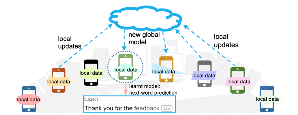
In my last post, I covered a high-level overview of Federated Learning, its applications, advantages & challenges.
We also went through a high-level overview of how Federated Optimization algorithms work. But from a mathematical sense, how is Federated Learning training actually performed? That’s what we will be looking at in this post.
There was a paper, Communication-Efficient Learning of Deep Networks from Decentralized Data by Google (3637 citations!!!), in which the authors had proposed a federated optimization algorithm called FedAvg and compared it with a naive baseline, FedSGD.
FedSGD
Stochastic Gradient Descent (SGD) had shown great results in deep learning. So, as a baseline, the researchers decided to base the Federated Learning training algorithm on SGD as well. SGD can be applied naively to the federated optimization problem, where a single batch gradient calculation (say on a randomly selected client) is done per round of communication.
The paper showed that this approach is computationally efficient, but requires very large numbers of rounds of training to produce good models.
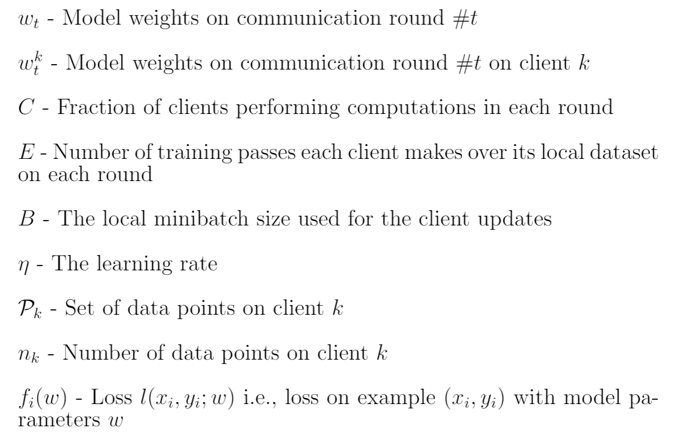
Before we get into the maths, I’ll define a few terms -
The baseline algorithm, was called FedSGD, short for Federated SGD.
For FedSGD, the parameter C (explained above) which controls the global batch size is set to 1. This corresponds to a full-batch (non-stochastic) gradient descent. For the current global model wt, the average gradient on its global model is calculated for each client k.
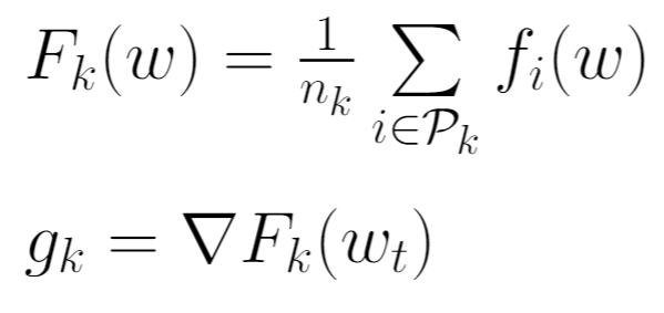
The central server then aggregates these gradients and applies the update.
FedAvg
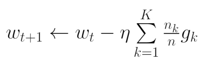
We saw FedSGD. Now let’s make a small change to the update step above.
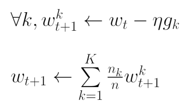
What this does is that now each client locally takes one step of gradient descent on the current model using its local data, and the server then takes a weighted average of the resulting models.
This way we can add more computation to each client by iterating the local update multiple times before doing the averaging step. This small modification results in the FederatedAveraging (FedAvg) algorithm.
But why make this change? The answer is in my last post -
In practice, major speedups are obtained when computation on each client is improved, once a minimum level of parallelism over clients is achieved.
The amount of computation is controlled by three parameters -
C - Fraction of clients participating in that round E - No. of training passes each client makes over its local dataset each round B - Local minibatch size used for client updates
The pseudocode for the FedAvg algorithm is shown below.
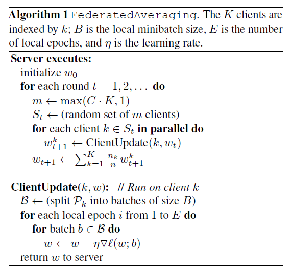
B = ꝏ (used in experiments) implies full local dataset is treated as the minibatch. So, setting B = ꝏ and E = 1 makes this the FedSGD algorithm.
Results
Okay, now let’s look at some experimental results, although I would also suggest looking up the results from the original paper as well. One experiment showed the number of rounds required to attain a target accuracy, in two tasks - MNIST and a character modelling task.
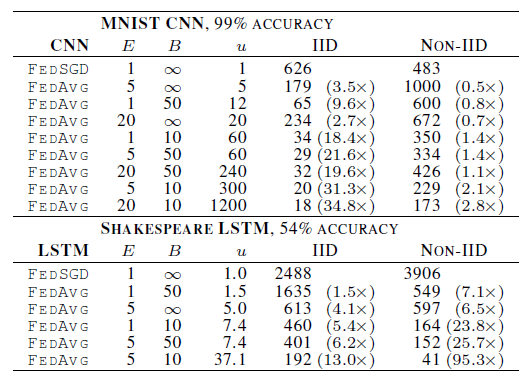
Here, IID and non-IID here refer to the datasets that were artificially generated by the authors to represent two kinds of distributions - IID, in which there is in fact an IID distribution among the clients. And non-IID in which the data is not IID among the clients. For example, for the MNIST dataset the authors studied two ways of partitioning the MNIST data over clients: IID, where the data is shuffled, and then partitioned into 100 clients each receiving 600 examples, and Non-IID, where we first sort the data by digit label, divide it into 200 shards of size 300, and assign each of 100 clients 2 shards. For the language modeling task, the dataset was built from The Complete Works of William Shakespeare. From the paper -
We construct a client dataset for each speaking role in each play with at least two lines. This produced a dataset with 1146 clients. For each client, we split the data into a set of training lines (the first 80% of lines for the role), and test lines (the last 20%, rounded up to at least one line). The resulting dataset has 3,564,579 characters in the training set, and 870,014 characters in the test set. This data is substantially unbalanced, with many roles having only a few lines, and a few with a large number of lines. Further, observe the test set is not a random sample of lines, but is temporally separated by the chronology of each play. Using an identical train/test split, we also form a balanced and IID version of the dataset, also with 1146 clients.
For the MNIST dataset, a CNN with two 5x5 convolution layers (the first with 32 channels, the second with 64, each followed with 2x2 max pooling), a fully connected layer with 512 units and ReLu activation, and a final softmax output layer was used. And for the language modeling task, a stacked character-level LSTM language model, which after reading each character in a line, predicts the next character. The model takes a series of characters as input and embeds each of these into a learned 8 dimensional space. The embedded characters are then processed through 2 LSTM layers, each with 256 nodes. Finally the output of the second LSTM layer is sent to a softmax output layer with one node per character. The full model has 866,578 parameters, and we trained using an unroll length of 80 characters.
From the results in the paper, it could be seen that in both the IID and non-IID settings, keeping a small mini-batch size and higher number of training passes on each client per round resulted in the model converging faster. For all model classes, FedAvg converges to a higher level of test accuracy than the baseline FedSGD models. For the CNN, the B = ꝏ; E = 1 FedSGD model reaches 99.22% accuracy in 1200 rounds, while the B = 10 ;E = 20 FedAvg model reaches an accuracy of 99.44% in 300 rounds.
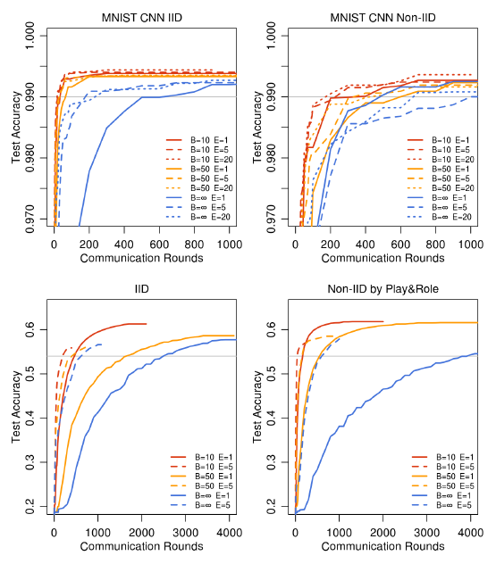
The authors also hypothesise that in addition to lowering communication costs, model averaging produces a regularization benefit similar to that achieved by dropout.
All in all, the experiments demonstrated that the FedAvg algorithm was robust to unbalanced and non-IID distributions, and also reduced the number of rounds of communication required for training, by orders of magnitude.
I wrote a Twitter thread on this topic as well - do give it a like/follow me if you liked the article.
My last thread covered a high-level overview of Federated Learning, its applications, advantages & challenges.
— Shreyansh Singh (@shreyansh_26) November 24, 2021
But from a mathematical sense, how is Federated Learning training actually performed? That's what we will be looking at in this thread 🧵https://t.co/anyvEluWoq
That’s the end for now!
This post finishes my summary on the basics of Federated Learning and is also a concise version of the very famous paper “Communication-Efficient Learning of Deep Networks from Decentralized Data” by Google.
I have also released an annotated version of the paper. If you are interested, you can find it here.
If the post helps you or you have any questions, do let me know!