Paper: Sophia: A Scalable Stochastic Second-order Optimizer for Language Model Pre-training
Link: https://arxiv.org/abs/2305.14342
Authors: Hong Liu, Zhiyuan Li, David Hall, Percy Liang, Tengyu Ma
Code: https://github.com/Liuhong99/Sophia

I have also released an annotated version of the paper. If you are interested, you can find it here.

---

Sophia is probably one of the most interesting papers I have read recently and I really liked how well it was written. This post is basically the notes that I had made while reading the paper, which is why it is not exactly a blog post and most of it is verbatim copied from the paper. But since there are a lot of optimization-theory related concepts which have been mentioned in the paper, I have tried to add my own set of references which I have read in the past that helped me understand the paper better. Hopefully it helps someone!

Overview

• The goal of this work is to propose a new optimizer for pre-training LLMs that can improve pre-training efficiency with a faster optimizer, which either reduces the time and cost to achieve the same pre-training loss, or alternatively achieves better pre-training loss with the same budget.

• Adam and its variants have become the somewhat default optimizers which are used in LLM pretraining.

• Designing fast optimizers for LLMs is challenging because -

  • The benefit of the first-order pre-conditioner (the $1/\sqrt{v_t}$ factor) in Adam is still not well understood.
  • The choice of pre-conditioners is constrained because we can only afford light-weight options whose overhead can be offset by the speed-up in the number of iterations.
  • Among the recent works on light-weight gradient-based pre-conditioners, Lion stood out as it is substantially faster than Adam on vision Transformers and diffusion models but only achieves limited speed-up on LLMs.

• This paper introduces Sophia, Second-order Clipped Stochastic Optimization, a light-weight second-order optimizer that uses an inexpensive stochastic estimate of the diagonal of the Hessian as a pre-conditioner and a clipping mechanism to control the worst-case update size.

• Key Results -

  

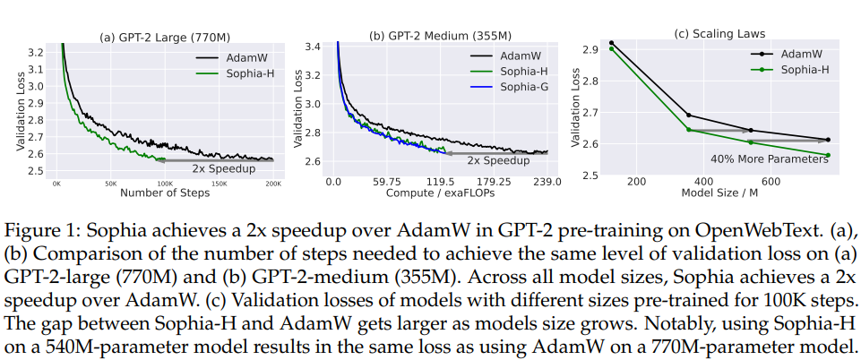
  • Sophia achieves the same validation pre-training loss with 50% fewer number of steps than Adam.
  • Sophia maintains almost the memory and average time per step and therefore the speedup also translates to 50% less total compute and 50% less wall-clock time.
  • The scaling law based on model size from 125M to 770M is in favor of Sophia over Adam - the gap between Sophia and Adam with 100K steps increases as the model size increases. Sophia on a 540M-parameter model with 100K steps gives the same validation loss as Adam on a 770M-parameter model with 100K steps.
    
    

• Checking the performance and scalability of this optimizer for pre-training much larger model sizes would (although expensive) be interesting to see.

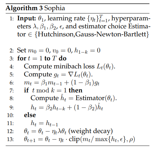
• Sophia estimates the diagonal entries of the Hessian of the loss using a mini-batch of examples every $k$ steps ($k=10$ in the paper).

• The paper considers two options for diagonal Hessian estimators -

  • Hutchinson’s unbiased estimator - an unbiased estimator that uses a Hessian-vector product with the same run-time as a mini-batch gradient up to a constant factor
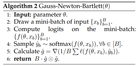
  • Gauss-Newton-Bartlett (GNB) estimator - a biased estimator that uses one mini-batch gradient calculated with resampled labels.
    
    

• Both the estimators introduce only a 5% overhead per step (on average).

• Sophia updates the parameter with an exponential moving average (EMA) of the gradient divided by the EMA of the diagonal Hessian estimate, subsequently clipped by a scalar.

• Due to the Hessian-based pre-conditioner, Sophia adapts more efficiently, than Adam does, to the heterogeneous curvatures in different parameter dimensions, which can often occur in the landscape of LLMs losses and cause instability or slowdown.

• In terms of the loss landscape, Sophia has a more aggressive pre-conditioner than Adam - Sophia applies a stronger penalization to updates in sharp dimensions (where the Hessian is large) than the flat dimensions (where the Hessian is small), ensuring a uniform loss decrease across all parameter dimensions. In contrast, Adam’s updates are mostly uniform across all parameter dimensions, leading to a slower loss decrease in flat dimensions.

• Sophia’s clipping mechanism controls the worst-case size of the updates in all directions, safeguarding against the negative impact of inaccurate Hessian estimates, rapid Hessian changes over time, and non-convex landscape.

Motivations

Heterogeneous Curvatures

• Loss functions in modern deep learning problems often have different curvatures across different parameter dimensions.
• The paper demonstrates the limitations of Adam and Gradient Descent by considering a two dimensional loss function - $L(\theta_{[1]},\theta_{[2]}) = L_1(\theta_{[1]}) + L_2(\theta_{[2]})$ where $$L_{1}(\theta_{[1]}) = 8(\theta_{[1]} - 1)^2(1.3\theta_{[1]}^2 + 2\theta_{[1]} + 1)$$ $$L_2(\theta_{[2]}) = 1/2 (\theta_{[2]} - 4)^2$$
• Here $L_1$ is much sharper than $L_2$.
• Another optimizer, SignGD is also compared which is quite old but can be understood as a simplified version of Adam, which does not involve taking the EMA for gradients and second moments of the gradients. The update then simplifies to - $\eta \cdot \nabla L(\theta)/|\nabla L(\theta)| = \eta\cdot \textup{sign}(\nabla L(\theta))$.

Limitations of GD and SignGD (Adam)

• The optimal learning rate of Gradient Descent should be proportional to the inverse of the curvature, i.e., the Hessian/second derivative at the local minimum. A good set of resources to understand this in detail are some notes from University of Toronto Section 2.2 and Section 4.1.
• So, if the curvatures of $L_1$ and $L_2$ at the local minima are $h_1$ and $h_2$ respectively (and thus $h_1 > h_2$ ). So the largest shared learning rate can only be $1/h_1$. Hence, the convergence in $\theta_{[2]}$ dimension is slow as also shown in the figure above.
  
  
• The update size of SignGD is the learning rate $\eta$ in all dimensions. Hence, intuitively, the same update size translates to less progress in decreasing the loss in the flat direction than in the sharp direction. In the yellow curve in the above figure, the progress of SignGD in the flat dimension $\theta_{[2]}$ is slow and along $\theta_{[1]}$, theiterate quickly travels to the valley in the first three steps and then starts to bounce. To fully converge in the sharp dimension, the learning rate $\eta$ needs to decay to $0$, which will exacerbate the slow convergence in the flat dimension $θ_{[2]}$. The trajectory of Adam is similar to SignGD and shown by the red curve in the figure.
  
  
• The behavior of SignGD and Adam above indicates that a more aggressive pre-conditioning is needed - sharp dimensions should have relatively smaller updates than flat dimensions so that the decrease of loss is equalized in all dimensions.
• Prior work on second order optimization suggest that the optimal pre-conditioner is the Hessian which captures the curvature on each dimension.
• The Newton’s method, does something similar - the update is the gradient divided by the Hessian in each dimension.$$\theta_{[1]} \leftarrow \theta_{[1]} - \eta \cdot L’_1(\theta_{[1]}) / h_1\ \ \textup{and}\ \ \theta_{[2]} \leftarrow \theta_{[2]} - \eta \cdot L’_2(\theta_{[2]})/ h_2$$
  

Limitations of Newton’s method

• Vanilla Newton’s method could converge to a global maximum when the local curvature is negative.
• As shown in the blue curve in the figure, Newton’s method quickly converges to a saddle point instead of a local minimum.
• Since the curvature may change rapidly along a trajectory, the second order information can often become unreliable.
  
  
• Sophia addresses this by considering only pre-conditioners that capture positive curvature, and introduce a per-coordinate clipping mechanism to mitigate the rapid change of Hessian. Applying those changes results in the following update - $$\theta_{[1]} \leftarrow \theta_{[1]} - \eta \cdot \textup{clip}(\frac{ L’_1(\theta_{[1]})}{\max{h_1,\epsilon}} ,\rho)\ \textup{and}\ \theta_{[2]} \leftarrow \theta_{[2]} - \eta \cdot \textup{clip}(\frac{ L’_2(\theta_{[2]})}{\max{h_2,\epsilon}},\rho)$$
• Here, $\rho$ is a constant to control the worst-case update size, $\epsilon$ is a very small constant (e.g., 1e-12) to avoid dividing by 0.
• The beauty here is that when the curvature of some dimension is rapidly changing or negative and thus the second-order information is misleading and possibly leads to a huge update before clipping, the clipping mechanism kicks in and the optimizer defaults to SignGD (even though this is sub-optimal for benign situations).
• The black curve in the figure starts off similarly to SignGD due to the clipping mechanism in the non-convex region, making descent opposed to converging to a local maximum. In the convex valley, it converges to the global minimum with a few steps.
• Compared with SignGD and Adam, it makes much faster progress in the flat dimension $\theta_{[2]}$ (because the update is bigger in dimension $\theta_{[2]}$), while avoiding bouncing in the sharp dimension $\theta_{[1]}$ (because the update is significantly shrunk in the sharp dimension $\theta_{[1]}$).

Sophia: Second-order Clipped Stochastic Optimization

EMA of diagonal Hessian estimates

• The diagonal Hessian estimates definitely have overheads, so it is computed at every $k$ steps.
• At every time step $t$, where $t \ \textup{mod} \ k = 1$, the estimator returns an estimate $h_t$ of the diagonal of the Hessian of the mini-batch loss.
• Similar to the gradient of the mini-batch loss function, the estimated diagonal Hessian can also have large noise.
• The EMA performed at every $k$ steps helps denoise the estimates. $$h_t = \beta_2 h_{t-k} + (1 - \beta_2) \hat{h}_{t} \ \textup{ if } t \ \mathrm{mod} \ k = 1 ; \textup{ else } h_t = h_{t-1}$$

Per-coordinate clipping

• I personally found this very innovative.
• As mentioned in the previous section, the inaccuracy of Hessian estimates and the change of Hessian along the trajectory can make the second-order information unreliable.
• $$\theta_{t+1} \leftarrow \theta_{t} - \eta_t \cdot \textup{clip}(m_t / \max{h_t,\epsilon}, \rho)$$
• When any entry of $h_t$ is negative, e.g., $h_t[i] < 0$, the corresponding entry in the pre-conditioned gradient $m_t[i]/\max{h_t[i],\epsilon} = m_t[i]/\epsilon$ is extremely large and has the same sign as $m_t[i]$, and thus $\eta\cdot \textup{clip}(m_t[i] / \max{h_t[i],\epsilon}, \rho) = \eta\rho\cdot \textup{sign}(m_t[i])$, which is the same as stochastic momentum SignSGD.
• Sophia uses stochastic momentum SignSGD as a backup when the Hessian is negative (or mistakenly estimated to be negative or very small.) We also note that t
• The clipping mechanism controls the worst-case size of the updates in all parameter dimensions to be at most $\rho$, which also improves the stability (which could be a severe issue for second-order methods).

Diagonal Hessian Estimators

• I’ll keep this section short and brief, for the simple reason that the math is extremely interesting but also a bit difficult to understand. So, I’ll add references to the best of my knowledge and I encourage the reader to go through them thoroughly.

Hutchinson’s unbiased estimator

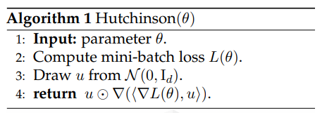
• For any loss function $\ell(\theta)$ on parameters $\theta\in \mathbb{R}^d$, the Hutchinson’s estimator can be used to obtain an unbiased estimator for the diagonal of the Hessian.
• First, draw $u\in \mathbb{R}^d$ from the spherical Gaussian distribution $\mathcal{N}(0,\mathrm{I}_d)$, and then output $\hat{h} = u \odot (\nabla^2 \ell(\theta) u)$, where $\odot$ denotes the element-wise product, and $\nabla^2 \ell(\theta) u$ is the HVP of the Hessian with $u$.
• Using HVP (from JAX or Pytorch allows us to efficiently compute the product of the Hessian and a vector without the actual computation of the full Hessian matrix.
• Effectively, $\mathbb{E}[\hat h] = \mathrm{diag}(\nabla^2 \ell(\theta))$.
  
  
• How does it work? The idea for the above comes from the original paper from Hutchinson - “A stochastic estimator of the trace of the influence matrix for Laplacian smoothing splines” which was about estimating the trace of a matrix. The idea there was -

  

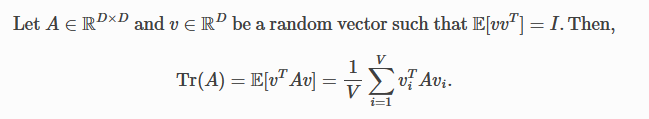
• Dimensionally, and somewhat intuitively, it kinda makes sense to change the dot product to an elementwise product to get the non-aggregated estimate of the diagonal (since trace is the sum of the diagonal elements).
• This idea was also used in the “Hessian Diagonal Approximation” section of the AdaHessian paper, and I would also encourage the reader to go through Section 2 of the paper - “An Estimator for the Diagonal of a Matrix”, which the AdaHessian paper cites as well.

Gauss-Newton-Bartlett (GNB) estimator

• The math for this section is particularly interesting and I would redirect you to my annotated paper where I have mentioned references and also worked out some of the math.
• I’d highly recommend reading Section 4.4 of these notes and optionally Section 4 of these notes (not absolutely required, just helps to understand the footnote in the Sophia paper).
• Ultimately, the GNB estimator used by the authors is $$B \cdot \nabla_\theta \widehat L(\theta) \odot \nabla_\theta \widehat L(\theta)$$ where $\widehat L(\theta) = \frac{1}{B}\sum_{b=1}^B \ce(f(\theta, x_b), \hat{y}_b)$, here $\hat{y}_b$ are not the labels corresponding to $x_b$. They are just __sampled labels__ from the mini-batch.
• The reason we can do that is in the math, which comes from the combination of
  1. The claim in the paper that the second-order derivative of the loss w.r.t. the logits only depends on the logits and the true labels $y$.
  2. Bartlett’s first identity, which generally holds for the negative log-likelihood loss of any probabilistic model and which states - $$\forall b, \mathbb{E}_{\hat{y}_b}\nabla L\textup{ce}(f(\theta,x_b),\hat{y}_b) = 0$$
• Also, the above estimator is an unbiased estimator for the diagonal of the Gauss-Newton matrix, which is a biased estimator for the diagonal of the Hessian.
• Additional References - Bartlett Identities

Comparison of Hessian estimators

• The Hutchinson’s estimator does not assume any structure of the loss, but requires a Hessian-vector product.
• The GNB estimator only estimates the Gauss-Newton term but always gives a positive semi-definite (non-negative) diagonal Hessian estimate. The PSDness ensures that the pre-conditioned update is always a descent direction.
• The Gauss-Newton Matrix is guaranteed to be PSD if the above-mentioned second-order derivative of the loss w.r.t. the logits is PSD. For proof, refer this.

Experiments

• There are tons of details in the paper regarding the experiments. I’ll just mention the key points here, just in case I have to look up something quickly.

Experimental Setup

Baselines

• Main comparison with AdamW and Lion
• AdamW for GPT2 hyperparams - WD = 0.1, $\beta_1 = 0.9$ and $\beta_2 = 0.95$
• Lion for GPT2 hyperparams - $\beta_1 = 0.95$ and $\beta_2 = 0.98$

Implementation

• Batch Size = 480
• Cosine LR schedule with the final LR equal to 0.05 times the peak LR
• Standard gradient clipping (by norm) threshold 1.0
• Fixed 2k steps of LR warm-up
• For Sophia, the authors use $\beta_1 = 0.96$, $\beta_2 = 0.99$, $\epsilon=$ 1e-12 and update diagonal Hessian every 10 steps.
• Sophia-H (which refers to Sophia with Hutchinson estimator) uses $\rho=0.01$, and only a subset of 32 examples from the mini-batch to calculate the diagonal Hessian to further reduce overhead.
• Sophia-G (which refers to Sophia with GNB estimator) uses $\rho=20$, and use a subset of 240 examples from the mini-batch to calculate the diagonal Gauss-Newton.
• All models are trained in bfloat16.
• The 125M and 355M models are trained on A5000 GPUs, while the 770M models are trained on A100 GPUs. Total amount of compute spent on all experiments is about 6000 hours on A100s and 10000 hours on A5000s. This amounts to 4.38e21 FLOPs.

Results

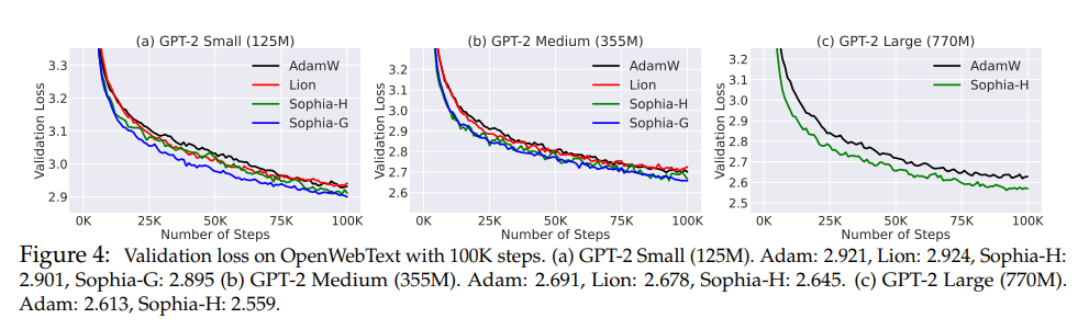
• Sophia consistently achieves better validation loss than AdamW and Lion.
• As the model size grows, the gap between Sophia and baselines also becomes larger. Sophia-H and Sophia-G both achieve a 0.04 smaller validation loss on the 355M model, Sophia-H achieves a 0.05 smaller validation loss on the 770M model with the same 100k steps.

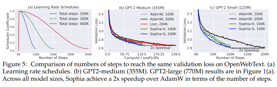
• According to the scaling laws in this regime, an improvement in loss of 0.05 is equivalent to 2x improvement in terms of number of steps or total compute to achieve the same validation loss
• Sophia is 2x faster in terms of number of steps, total compute and wall-clock time.
• The scaling law is in favor of Sophia-H over AdamW
  • The 540M model trained by Sophia-H has smaller loss than the 770M model trained by AdamW.
  • The 355M model trained by Sophia-H has comparable loss as the 540M model trained by AdamW.
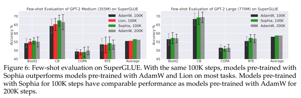
• Few-shot Evaluation on Downstream Tasks (SuperGLUE)

  

  • GPT-2 medium and GPT-2 large pre-trained with Sophia have better few-shot accuracy on most subtasks.
  • Models pre-trained with Sophia-H have comparable few-shot accuracy as models pre-trained with AdamW for 2x number of steps.
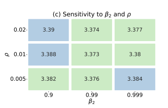
• Sensitivity to $\rho$ and $\beta_2$, and transferability of hyperparameters

  

  • While performing grid search on hyperparams on a smaller 30M model, the authors found that all combinations have a similar performance. Moreover, this hyperparameter choice is transferable across model sizes. For all the experiments on 125M, 355M and 770M, we use the hyperparameters searched on the 30M model, which is ρ = 0.01, β2 = 0.99.
• Training Stability
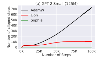
  • Gradient clipping (by norm) is an important technique in language model pre-training as it avoids messing up the moment of gradients with one mini-batch gradient computed from rare data.
  • In practice, the frequency that gradients clipping is triggered is related to the training stability - if the gradient is frequently clipped, the iterate can be in a very unstable state.

  

  • Although all methods use the same clipping threshold 1.0, Sophia-H seldomly triggers gradient clipping, while AdamW and Lion trigger gradient clipping in more than 10% of the steps
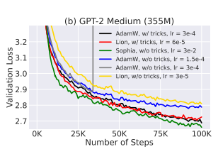
• Another common trick of pre-training deep Transformers is scaling the product of keys and values by the inverse of the layer index [Mistral]. This stabilizes training and increases the largest possible learning rate.

  

  • Without this trick, the maximum learning rate of AdamW and Lion on GPT-2 medium (355M) can only be 1.5e-4, which is much smaller than 3e-4 with the trick (the loss will blow up with 3e-4 without the trick). Moreover, the loss decreases much slower without the trick as shown. In all the experiments, Sophia-H does not require scaling the product of keys and values by the inverse of the layer index.

Limitations

• Scaling up to larger models and datasets
  • The paper only experiments with GPT-2 pretraining on OpenWebText for model sizes up to 770M params.
  • Although it is faster and better than Adam and Lion in these set of experiments, and the scaling laws and pre-training stability are encouraging, it remains to be seen how well Sophia scales on larger models.
• Holistic downstream evaluation
  • The paper has only experimented with 4 SuperGLUE tasks and although the results are encouraging, a better downstream evaluation is still important.
  • To note - The limitation in downstream evaluation is also due to the limited model size, because language models at this scale do not have enough capabilities such as in-context learning, and mathematical reasoning.
• Evaluation on other domains
  • This paper focuses on optimizers for LLMs, it should be evaluated in other domains like CV, RL and Multimodal tasks.

---

A very exciting paper. Hope people can test it out on even bigger models and across multiple domains and we may potentially have an optimizer finally dethroning Adam!

 

 

Follow me on Twitter, Github or connect on LinkedIn.