Paper Summary #13 - Physics of Language Models: Part 2.1, Grade-School Math and the Hidden Reasoning Process
Paper: Arxiv Link
Video: YouTube Link
Annotated Paper: Github repo
Key Questions
- Can language models truly develop reasoning skills, or do they simply memorize templates?
- What is the model’s hidden (mental) reasoning process?
- Do models solve math questions using skills similar to or different from humans?
- Do models trained solely on GSM8K-like datasets develop reasoning skills beyond those necessary for solving GSM8K problems?
- What mental process causes models to make reasoning mistakes?
- How large or deep must a model be to effectively solve GSM8K-level math questions?
Idea
- To study reasoning and intelligence, a pre-trained model can be fine-tuned on existing math problem datasets like GSM8K.
- However, there are concerns that GSM8K or similar data may be leaked in the pre-train data for LLMs.
- Hence when answering mathematical questions, it is hard to tell whether these models are actually performing reasoning (i.e. questions 1-3 above) or has just memorized problem templates during training.
- Using existing math datasets like GSM8K for pre-training is insufficient due to the small size of these datasets.
- Also, the idea of using GPT4 to augment similar problems like GSM8K wasn’t chosen because of the potential bias of the augmented data towards a small number of solution templates.
- Hence the authors created their own pre-training dataset of math problems, with a much larger and diverse set of grade-school math problems to test a GPT2-like language model.
Dataset Generation
- This section in the paper is super cool but also quiet dense.
- It is a great source of learning on how to create synthetic datasets. Won’t go into much detail in the notes, the paper is the best source to understand the complexity.
- A standard grade-school math problem in GSM8K looks like this -
-
Betty is saving money for a new wallet which costs 100. Betty has only half of the money she needs. Her parents decided to give her 15 for that purpose, and her grandparents twice as much as her parents. How much more money does Betty need to buy the wallet?
-
- This problem has multiple parameters whose values are connected with various equalities, such as “Betty’s current money = 0.5 × cost of the wallet” and “money given by grandparents = 2 × money given by parents.”
- Motivated by this, the authors build a GSM8K-like math dataset through a synthetic generation pipeline that captures the dependencies of parameters.
- The main focus was on the “logical reasoning” aspect of the problems which involves understanding the dependency of parameters in the problem statement, such as direct, instance, and implicit dependencies.
- Dependency Types:
- Direct Dependency: Parameters directly depend on others (e.g., \(A = 5 \times (X + Y)\)).
- Instance Dependency: Parameters depend on instances of categories (e.g., total number of chairs = chairs per classroom × number of classrooms).
- Implicit Dependency: Parameters involve abstract concepts that need to be inferred (e.g., identifying fruits from a list of items).
- Problem Structure: Problems are generated using a hierarchical categorization of items, where each category can include multiple layers and items. This structure adds complexity by requiring models to learn concepts implicitly.
- Dependency Graph: A directed acyclic graph (DAG) is used to represent dependencies among parameters, including both direct and implicit dependencies. The graph guides the generation of math problems by linking parameters in specific ways.
- Problem Generation: The math problems are articulated by translating the dependency graphs into English sentences. The order of these sentences is randomized to increase the difficulty, and a question is posed to test the model’s understanding.
- Additional care was taken to reduce the difficulty of the problem statements
- Ensuring clarity in expression, to reduce the difficulty arising from common-sense
- For arithmetic, all integers and arithmetic were mod23
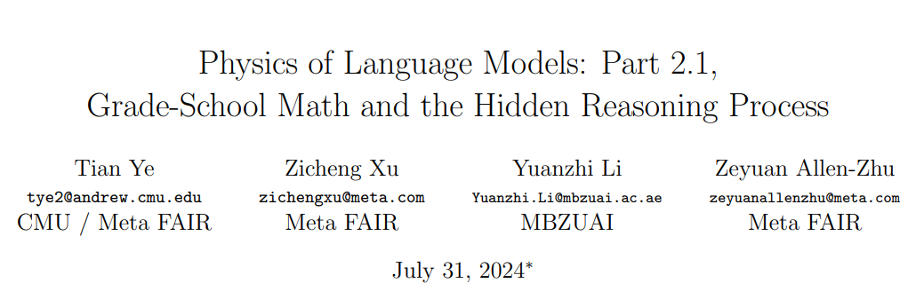
- A sample problem (corresponding to the figure above) looks like this -
-
The number of each Riverview High’s Film Studio equals 5 times as much as the sum of each Film Studio’s Backpack and each Dance Studio’s School Daypack. The number of each Film Studio’s School Daypack equals 12 more than the sum of each Film Studio’s Messenger Backpack and each Central High’s Film Studio. The number of each Central High’s Film Studio equals the sum of each Dance Studio’s School Daypack and each Film Studio’s Messenger Backpack. The number of each Riverview High’s Dance Studio equals the sum of each Film Studio’s Backpack, each Film Studio’s Messenger Backpack, each Film Studio’s School Daypack and each Central High’s Backpack. The number of each Dance Studio’s School Daypack equals 17. The number of each Film Studio’s Messenger Backpack equals 13. How many Backpack does Central High have?
-
Solution Construction
- The solution generation is done in the Chain of Thought reasoning format.
- The methodology is given below -
- Let solution be a sequence of sentences describing the necessary steps towards solving the given problem, where the sentences follow any topological order - known as CoT
- For each parameter necessary towards answering the final question, it is assigned a random letter among the 52 choices (a..z or A..Z), and a sentence is used to describe its computation.
- Sample solution corresponding to the above problem -
-
Define Dance Studio’s School Daypack as p; so p = 17. Define Film Studio’s Messenger Backpack as W; so W = 13. Define Central High’s Film Studio as B; so B = p + W = 17 + 13 = 7. Define Film Studio’s School Daypack as g; R = W + B = 13 + 7 = 20; so g = 12 + R = 12 + 20 = 9. Define Film Studio’s Backpack as w; so w = g + W = 9 + 13 = 22. Define Central High’s Backpack as c; so c = B * w = 7 * 22 = 16. Answer: 16.
- Important points during solution construction -
- The solution only contain parameters necessary towards calculating the final query parameter
- The solution follows the correct logical order: i.e. all the parameters used in the calculation must have appeared and been computed beforehand.
- Computations are broken into binary ops: \(g = 12 + 13 + 7\) is broken into g = 12+R and R = 13+7 in the above solution. The number of semicolons “;” equals the number of operations. This reduces the arithmetic complexity of the solution.
Difficulty Control
- Two parameters are used to control the difficulty of the problem -
- \(\textrm{ip}\) is the number of instance parameters
- \(\textrm{op}\) is the number of solution operations
- The data difficulty is an increasing function over them
- The authors call the dataset iGSM
- We use \(\textrm{iGSM}^{\textrm{op} \leq op,\textrm{ip} \leq ip}\) to denote the data generated with constraint \(\textrm{op} \leq op\) and \(\textrm{ip} \leq ip\), and use \(\textrm{iGSM}^{\textrm{op}=op,\textrm{ip} \leq ip}\) to denote those restricting to \(\textrm{op}=op\).
Train and Test Datasets
- \(\textrm{iGSM-med}\) uses \(\textrm{ip} \leq 20\)
- Train data is essentially \(\textrm{iGSM}^{\textrm{op} \leq 15,\textrm{ip} \leq 20}\) (referred as \(\textrm{iGSM-med}^{\textrm{op} \leq 15}\))
- Evaluation is done on both \(\textrm{iGSM-med}^{\textrm{op} \leq 15}\) and out-of-distribution (OOD) on \(\textrm{iGSM-med}^{\textrm{op} \leq op}\) where \(op \in \{20, 21, 23, 23\}\)
- Another set of evaluation is also done on \(\textrm{iGSM-med}^{\textrm{op} = op,\textrm{reask}}\). Here \(\textrm{reask}\) denotes first generating a problem from \(\textrm{iGSM-med}^{\textrm{op} = op}\) and then resampling a query parameter.
- Due to the topological nature of the data/solution generation process, \(\textrm{reask}\) greatly changes the data distribution and the number of operations needed. It provides an excellent OOD sample for evaluation.
- \(\textrm{iGSM-hard}\) uses \(\textrm{ip} \leq 28\)
- Train data is essentially \(\textrm{iGSM}^{\textrm{op} \leq 21,\textrm{ip} \leq 28}\) (referred as \(\textrm{iGSM-hard}^{\textrm{op} \leq 21}\))
- Evaluation is done on both \(\textrm{iGSM-hard}^{\textrm{op} \leq 21}\) and out-of-distribution (OOD) on \(\textrm{iGSM-hard}^{\textrm{op} \leq op}\) where \(op \in \{28, 29, 30, 31, 32\}\)
- Another set of evaluation is also done on \(\textrm{iGSM-hard}^{\textrm{op} = op,\textrm{reask}}\).
- Key points about the dataset
- Ignoring unused parameters, numerics, sentence orderings, English words, a-z and A-Z letter choices, \(\textrm{iGSM}^{\textrm{op} = 15}\) still has at least 7 billion solution templates, and \(\textrm{iGSM-hard}^{\textrm{op} = 21}\) has at least 90 trillion solution templates.
- The OOD evaluation is guaranteed to not have data contamination as training is done only on \(\textrm{op} \leq 21\) but evaluation is done on \(\textrm{op} \geq 28\)
- Training is done on data whose hash value of solution template is \(<17\) (mod 23), and but tested with those \(\geq 17\). This ensures no template-level overlap between training and testing.
Model
- A GPT2 model but with its positional embedding replaced with rotary embeddings (RoPE)
- It is still called GPT2 in the paper
- The authors mostly stick to the 12-layer, 12-head, 768-dim GPT2 (a.k.a. GPT2-small, 124M) for experiments but also explore larger models for some experiments
- The context length is 768 / 1024 for pretraining on \(\textrm{iGSM-med}\) / \(\textrm{iGSM-hard}\) and 2048 for evaluation.
Key Result - Model’s Behavior process
- TL;DR -
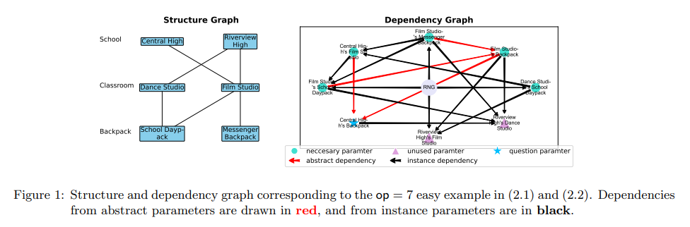
- The authors demonstrate that the GPT2 model, pretrained on the synthetic dataset, not only achieves 99% accuracy in solving math problems from the same distribution but also out-of-distribution generalizes, such as to those of longer reasoning lengths than any seen during training.
- Note that the model has never seen any training example of the same length as in test time.
- This signifies that the model can truly learn some reasoning skill instead of memorizing solution templates.
- Crucially, the model can learn to generate shortest solutions, almost always avoiding unnecessary computations.
- This suggests that the model formulates a plan before it generates, in order to avoid computing any quantities that are not needed towards solving the underlying math problem.
Key Result - Model’s Mental Process
- TL;DR
- The authors examine the model’s internal states through probing, introducing six probing tasks to elucidate how the model solves math problems.
- For instance, they discover that the model (mentally!) preprocesses the full set of necessary parameters before it starts any generation. Likewise, humans also do this preprocess although we write this down on scratch pads.
- The model also learns unnecessary, yet important skills after pretraining, such as all-pair dependency.
- Before any question is asked, it already (mentally!) computes with good accuracy which parameters depend on which, even though some are not needed for solving the math problem.
- Note that computing all-pair dependency is a skill not needed to fit all the solutions in the training data. This is the first evidence that a language model can learn useful skills beyond those necessary to fit its pretraining data.
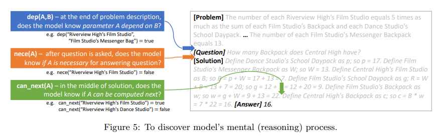
- The authors use linear probing to study the following tasks which align with human problem-solving strategies -
- \(\textrm{nece(A)}\): If the parameter \(A\) is necessary for computing the answer.
- \(\textrm{dep(A, B)}\): if parameter \(A\) (recursively) depends on parameter B given the problem statement.
- \(\textrm{known(A)}\): if parameter \(A\) has already been computed.
- \(\textrm{value(A)}\): the value of parameter \(A\) (a number between 0-22, or 23 if \(\textrm{known(A) = false}\)).
- \(\textrm{can_next(A)}\): if \(A\) can be computed in the next solution sentence (namely, its predecessors have all been calculated). Note that \(A\) might not be necessary to answer the question.
- \(\textrm{nece_next(A)}\): if parameter A satisfies both \(\textrm{can_next(A)}\) and \(\textrm{nece(A)}\).
- For a model to generate the shortest solutions, it must identify \(\textrm{nece(A)}\) for all \(A\)’s in its mental process.
- Whether \(\textrm{nece(A)}\) is \(\textrm{true}\), directly corresponds to whether there is a solution sentence to compute \(A\).
- Other similar probing tasks and what they imply are shown in the figure below -
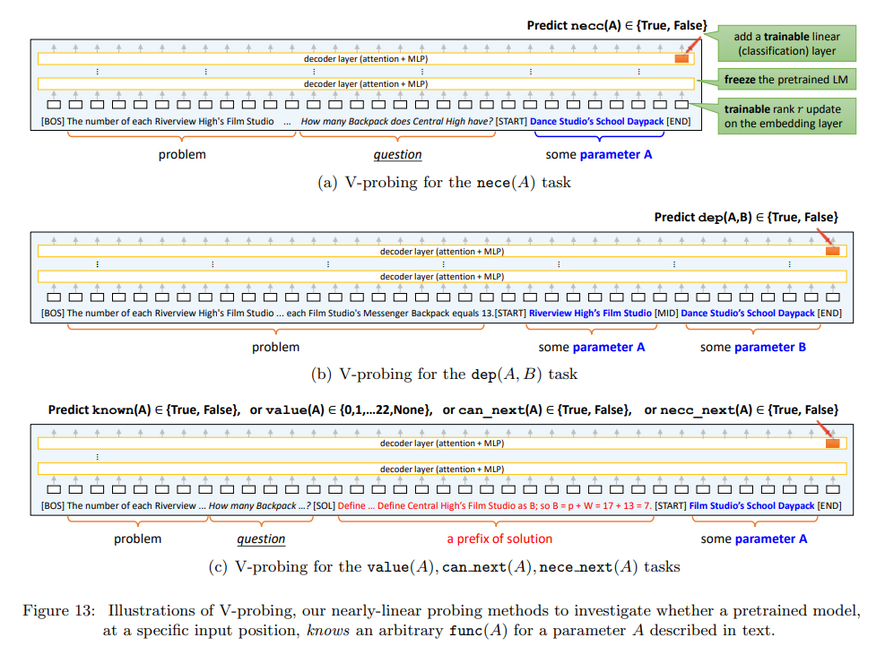
V(ariable)-Probing: A Nearly-Linear Probing Method
- As illustrated in the figure above, the authors conduct probing
- At the end of the problem description for the \(\textrm{dep}\) task
- At the end of the question description for the \(\textrm{nece}\) task
- For all other tasks, they are probed at the end of every solution sentence
- In Linear Probing a trainable linear classifier is introduced over the hidden states and a lightweight finetuning is performed for the task.
- V-Probing however has certain differences.
- Motivation: V-Probing is introduced to handle more complex properties in math problems that involve one or two conditional variables (A and B) described in plain English.
- Probing Setup: The math problems are truncated to the probing position, and special tokens
[START]and[END]are placed around the descriptions of A (or A, B). The probing is done from the[END]token position to check if the property is linearly encoded in the model’s last layer. - Enhancement Over Linear Probing: Unlike standard linear probing, V-Probing introduces a small, trainable rank-8 linear update to the input embedding layer to account for input changes.
- Training Process: The pretrained language model is frozen, and both the linear classifier and the rank-8 update are fine-tuned to probe for the desired property, making the process more adaptable to complex input structures.
Probing Results
- The probing accuracies are high for all the tasks, compared to majority guess and random-model probing - except for the very hard OOD cases (i.e., for large op where the model’s generation accuracies fall down to 80% anyways.
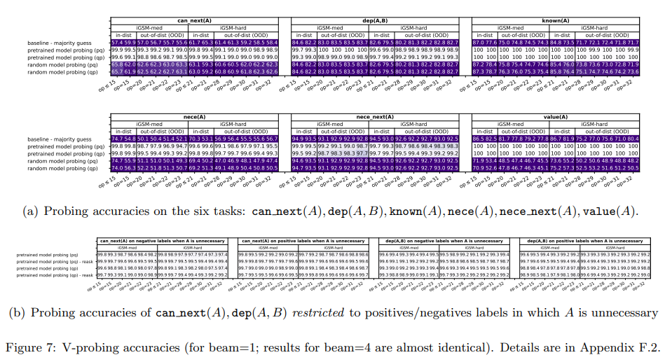
- Model solves math problems like humans
- When generating solutions, the model not only remembers which parameters have been computed and which have not (\(\textrm{value, known}\)) but also knows which parameters can be computed next (\(\textrm{can_next, nece_next}\)). These abilities ensure that the model can solve the given math problem step by step, similar to human problem-solving skill.
- By the end of the problem description, the model already knows the full list of necessary parameters (\(\textrm{nece}\)). This indicates that the model has learned to plan ahead, identifying necessary parameters before starting to generate the solution. This aligns with human behavior, except that the model plans mentally while humans typically write this down.
- Model learns beyond human reasoning skills
- The model learns \(\textrm{dep(A, B)}\) and \(\textrm{can_next(A)}\), even for parameters A not necessary for answering the question, as shown in the figure above.
- This differs from human problem-solving, where we typically use backward reasoning from the question to identify necessary parameters, often overlooking unnecessary ones.
- In contrast, language models can pre-compute the all-pair dependency graph \(\textrm{dep(A, B)}\) mentally even before a question is asked. This “level-2” reasoning is very different from human behavior or mental processes.
- This enables the model to sort relationships among the things it hears, a skill that can be useful for future tasks (via instruction fine-tuning).
- This may be the first evidence of a language model acquiring skills beyond those needed for learning its pretrain data.
Key Results - Explain Model’s Mistakes
- The authors tried to answer the following questions -
- When does the model answer correctly but include unnecessary parameters?
- What causes incorrect answers?
- The aim is to determine if such erroneous behaviour of the model aligns with errors in the model’s mental process (via probing)
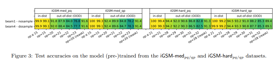
- Earlier, it was shown that the model rarely produces solutions longer than necessary, so the authors looked at the OOD \(\textrm{reask}\) data for evaluation.
- On this data, pretrained models produce an average of ~0.5 unnecessary parameters per solution even for \(\textrm{op} = 32\) (figure 4).
- The authors examined if these unnecessary parameters \(A\) were incorrectly predicted as \(\textrm{nece = true}\) in the probing task.
- The following figure reveals that this is often indeed the case, thus language models produce solutions with unnecessary steps due to errors in their mental planning phase.
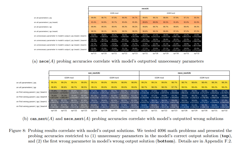
- In the second part of the figure, the author’s findings show that the model’s errors mainly stem from incorrectly predicting \(\textrm{nece_next(A)}\) or \(\textrm{can_next(A)}\) as true in its internal states when such \(A\)’s are not ready for computation.
- Essentially,
- Many reasoning mistakes made by the language model are systematic, stemming from errors in its mental process, not merely random from the generation process.
- Some of the model’s mistakes can be discovered by probing its inner states even before the model opens its mouth (i.e., before it says the first solution step).
Key Results - Depth vs. Reasoning Length
- The authors find that - Language model depth is crucial for mathematical reasoning.
- They experimented with model of various depths and various hidden sizes.
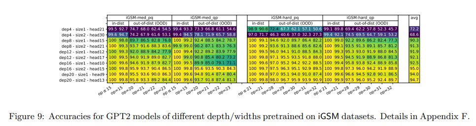
- From the figure above, it can be seen that a 4-layer transformer, even with 1920 hidden dimensions, underperforms on the math datasets in the paper.
- Conversely, deeper but smaller models, such as a 20-layer 576-dim, perform very well.
- There is a clear correlation between the model depth and performance.
But how does model depth influence math problem solving skills?
- Using the \(\textrm{nece}\) probing task, the authors focus on the necessary parameters at distance \(t\) from the query parameter, for \(t \in \{1,2,...,8\}\).
- Though these parameters all have \(\textrm{nece = true}\), but the model can be probed to see how correct they are at predicting \(\textrm{nece(A)}\) at different hidden layers.
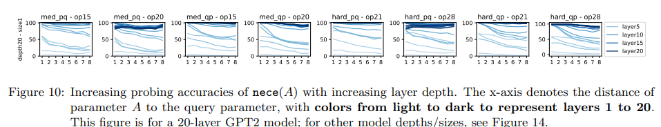
- The above figure shows a correlation between the model’s layer hierarchy, reasoning accuracy and mental reasoning depth.
- Shallower layers excel at predicting nece(A) for parameters \(A\) closer to the query, whereas deeper layers are more accurate and can predict \(\textrm{nece(A)}\) for parameters further from the query.
- This suggests that the **model employs layer-by-layer reasoning during the planning phase to recursively identify all parameters the query depends on. **
- So, for larger \(t\), the model may require and benefit from deeper models (assuming all other hyperparameters remain constant).
- To note -
- If the “backward thinking process” is added as CoT to the data, then deep mental thinking is no longer required, reducing the language model’s depth requirement. However, in practice, many such “thinking processes” may not be included in standard math solutions or languages in general.
- The above claim does not imply that “a \(t\)-step mental thinking requires a depth-\(t\) transformer”. It is plausible for a single transformer layer (containing many sub-layers) to implement \(t > 1\) mental thinking steps, though possibly with reduced accuracy as \(t\) increases. There is no exact correlation as it depends on the data distribution.