Deep dive into CUDA Scan Kernels: Hierarchical and Single-Pass Variants
The source code for this post is available on GitHub.
Introduction
A scan (prefix sum) is a deceptively small primitive: given an input array X, produce an output array Y where Y[i] = X[0] + X[1] + … + X[i]. On the GPU this is hard to do efficiently because each output depends on all previous elements, which sounds serial. The kernels in this repository explore multiple ways to restructure this computation so that thousands of threads can participate without breaking correctness.
There are two broad families here:
- Hierarchical (multi-pass) scans: scan within blocks, scan the block totals, then redistribute those totals back into the output. This is the most standard GPU scan strategy and maps cleanly to CUDA’s execution model.
- Single-pass scans: attempt to compute the full array scan in a single kernel launch using inter-block coordination (domino propagation or decoupled lookbacks). These are more complex but avoid extra kernel launches.
A CUB baseline in src/cub_scan.cu uses cub::DeviceScan::InclusiveSum as a reference for performance and correctness.
Quick CUDA primer (for context)
If you are new to CUDA, three concepts show up repeatedly in the kernels below:
- Warps: threads are executed in groups of 32. Many performance optimizations (like warp shuffles) are designed around this unit.
- Shared memory: fast, on-chip memory shared by threads in a block. Most scan algorithms use shared memory for their per-block scan stages.
- Synchronization:
__syncthreads()synchronizes threads within a block. There is no built-in global synchronization across blocks inside a kernel, which is why single-pass scans must use explicit memory protocols to coordinate.__threadfence()orders a thread’s global memory writes so they are visible to other threads/blocks on the device before it continues.
You’ll also see the term coalesced memory access. A global memory access is coalesced when consecutive threads in a warp access consecutive addresses, allowing the GPU to serve the warp with fewer memory transactions. This is a major performance factor, and it strongly influences how the kernels index into memory.
Hierarchical Scan Algorithms
Idea of hierarchical scan
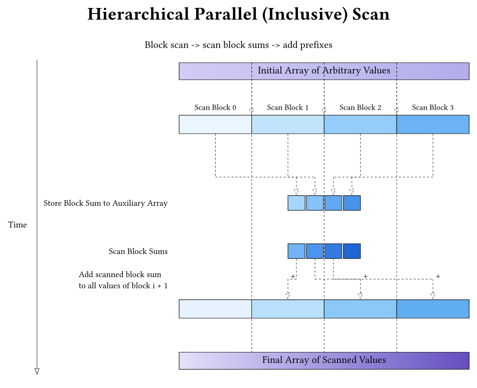
Hierarchical scan decomposes the full scan into three stages that are easy to parallelize:
- Per-block scan: each block scans a contiguous chunk of the input and writes the prefix results for that chunk into the output array. Each block also emits one number: the block total (sum of its entire chunk).
- Scan the block totals: scan the array of block totals to produce a prefix over blocks. Block 0 adds 0; block \(b>0\) adds the scanned total of block \(b-1\) (i.e., the sum of everything before block \(b\)). If this array is long, it is scanned hierarchically using multiple levels.
- Redistribution (add carry‑in): each block adds its carry‑in to every element of its local output, turning a block-local prefix into a correct global prefix.
In the source, the “block totals” buffer is called partialSums: it is an auxiliary array with one entry per thread block.
Concretely, after stage 1 each block has computed the right prefix order relative to the start of its own chunk, but every block except block 0 is missing a constant offset (the sum of all earlier chunks). Scanning the block totals computes exactly those offsets.
Example with BLOCK_SIZE = 4:
Input:        [1 2 3 4 | 5 6 7 8]
Local scans:  [1 3 6 10 | 5 11 18 26]
Block totals: [10, 26]
Scan totals:  [10, 36]
Add carry-in: [1 3 6 10 | (5+10) (11+10) (18+10) (26+10)]
            = [1 3 6 10 | 15 21 28 36]
This structure is consistent across:
src/hierarchical_kogge_stone*.cusrc/hierarchical_brent_kung*.cusrc/hierarchical_warp_tiled*_optimized.cu
A key idea for readers: the per-block scan only handles a local segment. The global correctness comes from the second and third stages, which propagate block totals across the array.
When the block-totals scan needs multiple levels
Stage 2 scans one value per block. If each block handles \(B =\) BLOCK_SIZE input elements, then the number of blocks is \(M = \lceil N / B \rceil\), so the block-totals array has length \(M\).
A single CUDA block in these kernels scans at most \(B\) values (one value per thread in shared memory), so stage 2 is:
- one-block when \(M \le B\) (equivalently \(N \le B^2\); for \(B = 1024\), about one million elements),
- a small recursive hierarchy when \(M > B\).
Conceptually, you build a short “pyramid” of group totals:
- Level 0: per-block totals (length \(M_0 = M\))
- Level 1: totals of contiguous groups of \(B\) entries from level 0 (length \(M_1 = \lceil M_0 / B \rceil\))
- …
- stop at the first level \(L\) with \(M_L \le B\)
Then you run the same up/down structure across levels:
- Up-sweep: scan each level in block-sized segments and write each segment’s total into the next level.
- Top scan: scan the final level in one block.
- Down-sweep: propagate prefixes back down by adding the scanned prefix of earlier segments (the carry‑in) into every element of the lower level.
In src/hierarchical_kogge_stone.cu, this logic is packaged as ScanLevels: level 0 is the block-totals buffer (partialSums in the code), and higher levels are temporary allocations that shrink by ~1024× each step:
while (curr_len > BLOCK_SIZE) {
    unsigned int next_len = cdiv(curr_len, BLOCK_SIZE);
    T* sums_d = nullptr;
    CHECK_CUDA_ERROR(cudaMalloc(&sums_d, next_len * sizeof(T)));
    levels.data.push_back(sums_d);
    levels.lengths.push_back(next_len);
    curr_len = next_len;
}
The scan then follows the “up-sweep / top / down-sweep” pattern literally:
for (size_t level = 0; level + 1 < levels.data.size(); ++level) {
    unsigned int len = levels.lengths[level];
    dim3 gridSize(cdiv(len, BLOCK_SIZE));
    kogge_stone_segmented_scan_kernel<<<gridSize, blockSize>>>(
        levels.data[level], levels.data[level], levels.data[level + 1], len);
}

kogge_stone_scan_kernel<<<dim3(1), blockSize>>>(
    levels.data.back(), levels.lengths.back());

for (int level = static_cast<int>(levels.data.size()) - 2; level >= 0; --level) {
    unsigned int len = levels.lengths[level];
    dim3 gridSize(cdiv(len, BLOCK_SIZE));
    redistribute_sum<<<gridSize, blockSize>>>(
        levels.data[level], levels.data[level + 1], len);
}
Without this multi-level pass, stage 2 would only produce correct prefixes within groups of \(B\) blocks, and the final redistribution would be wrong for long inputs.
Inclusive scan, padding, and boundaries
These kernels implement inclusive scan (each output includes its own input). That means the first output is just X[0]. For partial blocks at the end of the array, out-of-range elements are padded with the additive identity (0) so the tree logic stays correct. You’ll see code like:
XY_s[threadIdx.x] = (i < N) ? X[i] : static_cast<T>(0);
This padding is a simple but important trick: it keeps the scan math valid without branching the tree structure.
Kogge-Stone scan (simple)
Kernel: src/hierarchical_kogge_stone.cu
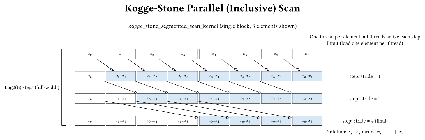
Kogge-Stone is the classic parallel scan. It uses a shared-memory array of size B (one element per thread), and performs log2(B) steps. In each step, every thread reads from a neighbor at distance stride and updates its own value. This produces an inclusive scan.
Core pattern (in-place):
for (unsigned int stride = 1; stride < blockDim.x; stride *= 2) {
    __syncthreads();
    T temp;
    if (threadIdx.x >= stride) {
        temp = XY_s[threadIdx.x] + XY_s[threadIdx.x - stride];
    }
    __syncthreads();
    if (threadIdx.x >= stride) {
        XY_s[threadIdx.x] = temp;
    }
}
Why two barriers per stride? Because updates are in-place: if thread i writes early, thread i+stride could see updated data incorrectly in the same stride. The temp + double barrier pattern avoids read-after-write hazards.
This file is the best place to start if you want to understand the baseline hierarchical scan flow end-to-end.
Key characteristics:
- Work: \(O(N \log N)\) additions
- Depth: \(\log_2(N)\) parallel steps
- Synchronization: Two
__syncthreads()per iteration (read-modify-write pattern) - Shared memory: \(B\) elements (where B is block size)
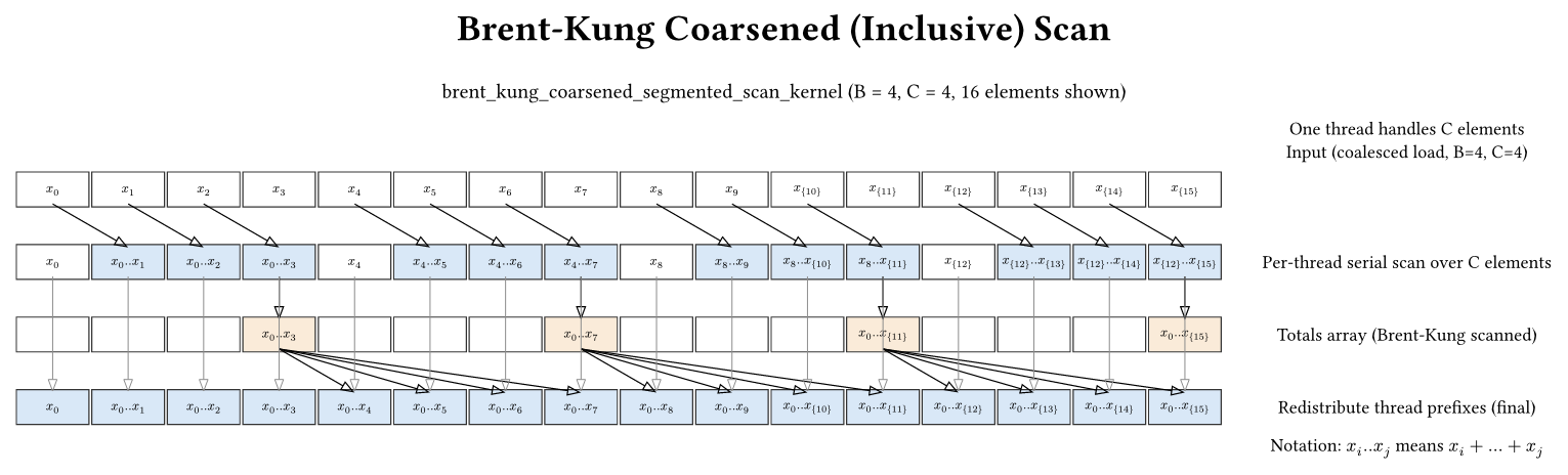
Kogge-Stone scan (coarsened)
Kernel: src/hierarchical_kogge_stone_coarsening.cu
Coarsening is a standard optimization: instead of one element per thread, each thread processes multiple elements. This reduces the number of blocks, which shrinks the block-totals buffer (partialSums) and thus reduces the amount of hierarchical work. It also increases the work per thread, which can improve instruction-level parallelism.
Why coalescing matters here
If each thread loaded a contiguous segment for itself, global memory access would be strided across threads and would not coalesce well. To preserve coalescing, the kernel loads/stores in the pattern:
- Coalesced layout:
data[c * B + t](consecutive threads read consecutive addresses)
But for the scan itself, each thread wants a contiguous segment. So the kernel reinterprets the shared memory layout as:
- Thread-major layout:
data[t * C + c]
This is effectively a shared-memory transpose: coalesced global access on the way in and out, but contiguous per-thread access during the scan. It’s one of the most common CUDA tricks for marrying coalescing with local contiguity.
If you want a concrete picture, imagine B = 8 and C = 2. A coalesced load makes threads read: thread 0 → X[0], thread 1 → X[1], … thread 7 → X[7], then again X[8..15] for c = 1. That is perfectly coalesced. But thread 0’s logical segment is X[0], X[1] (contiguous), which now sits in shared memory at positions data[0] and data[8]. The transpose reinterpretation is what makes that segment look contiguous again during the scan without sacrificing coalescing on the global load/store.
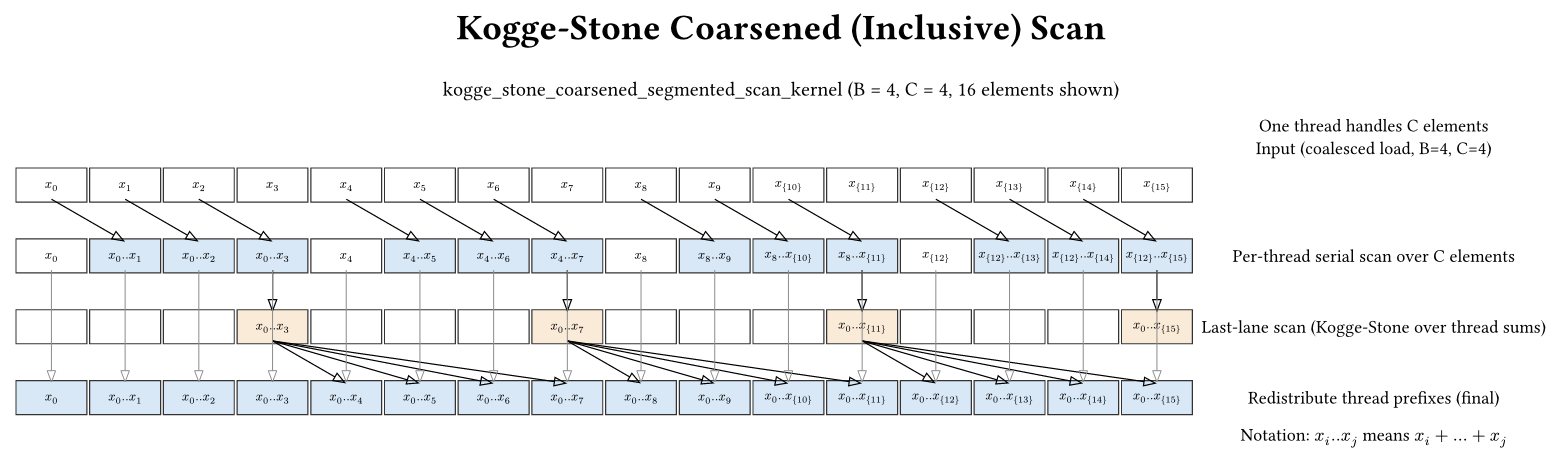
Scan flow:
- Each thread serially scans its C elements.
- Run a Kogge-Stone scan over the thread totals (last lane per thread).
- Redistribute each thread’s prefix to its remaining lanes.
The redistribution step is mandatory because of the shared-memory layout:
if (threadIdx.x > 0) {
    T add = XY_s[(threadIdx.x - 1) * COARSENING_FACTOR + (COARSENING_FACTOR - 1)];
    for (int c = 0; c < COARSENING_FACTOR - 1; ++c) {
        XY_s[threadIdx.x * COARSENING_FACTOR + c] += add;
    }
}
In contrast, some single-pass variants that keep the coarsened segment in registers can apply the redistribution implicitly at write-out time (see src/single_pass_scan_naive.cu). The explicit redistribution loop here is the price paid for the coalesced/shared-transpose layout.
Kogge-Stone scan (double buffering)
Kernel: src/hierarchical_kogge_stone_double_buffering.cu
Double buffering uses two shared-memory arrays. Each stride writes into the output buffer, then swaps input and output. That reduces synchronization to one barrier per stride:
out_XY_s[threadIdx.x] = (threadIdx.x >= stride)
    ? in_XY_s[threadIdx.x] + in_XY_s[threadIdx.x - stride]
    : in_XY_s[threadIdx.x];
__syncthreads();
T* temp = in_XY_s;
in_XY_s = out_XY_s;
out_XY_s = temp;
This often helps Kogge-Stone because the in-place version needs two barriers per stride, and Kogge-Stone has many strides (log2(B)). The extra shared-memory traffic is usually offset by fewer synchronizations.
Brent-Kung scan (simple)
Kernel: src/hierarchical_brent_kung.cu
Brent-Kung trades fewer total operations for a more complex indexing pattern. It scans 2B elements per block by assigning two elements per thread and building a balanced tree:
- Upsweep: reduce to a block total.
- Downsweep: distribute partial sums.
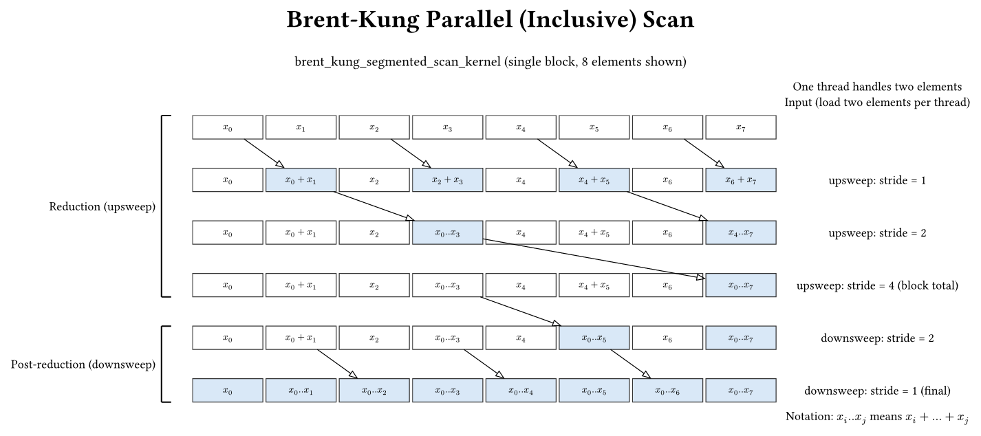
Unlike Kogge-Stone, Brent-Kung does not update all elements each stride; it updates only a subset. This is why its in-place version is efficient: it needs only one barrier per stride and does not require the temp + double barrier pattern.
Brent-Kung is often discussed as an algorithm with fewer operations but more complex indexing. In practice, the actual performance depends on shared-memory traffic and synchronization, which this codebase makes easy to study side-by-side.
Key characteristics:
- Work: \(O(N)\) additions (work-efficient)
- Depth: \(2\log_2(N)\) parallel steps
- Synchronization: One
__syncthreads()per iteration - Shared memory: \(2B\) elements
Brent-Kung scan (coarsened)
Kernel: src/hierarchical_brent_kung_coarsening.cu
The coarsened Brent-Kung kernel mirrors the Kogge-Stone coarsening idea, but with one extra detail: it uses a 2B shared array for the thread totals.
Why? The Brent-Kung scan kernel in this repository is written for an array of length 2 * blockDim, with two elements per thread. To reuse that exact kernel, the coarsened version pads the totals array:
- totals[0..B-1] = per-thread totals
- totals[B..2B-1] = 0
This preserves the expected tree shape and makes the existing Brent-Kung scan code correct without rewriting it.
After the totals scan, each thread adds the scanned total of all previous threads to its local \(C\) elements to produce the correct block-wide prefix order. This is the same “redistribution” idea as in coarsened Kogge-Stone, but the padded 2B array is a specific quirk of the Brent-Kung implementation here.
Brent-Kung scan (double buffering)
Kernel: src/hierarchical_brent_kung_double_buffering.cu
Brent-Kung double buffering is included for completeness, but it is usually not beneficial. The in-place Brent-Kung already avoids read-after-write hazards and uses one barrier per stride. The double-buffered version:
- Copies the entire 2B array each stride,
- Uses extra barriers,
- Doubles shared memory usage.
So the overhead outweighs the benefit for Brent-Kung in this codebase.
Optimized hierarchical scan (warp primitives + register tiling)
Kernels:
These optimized kernels combine multiple techniques to reduce synchronization and shared-memory traffic.
1) Warp-level inclusive scan
Instead of a block-wide shared-memory tree, each warp scans its own totals with warp shuffle primitives:
__device__ __forceinline__ T warp_inclusive_scan(T val, int lane) {
    unsigned int mask = 0xffffffff;
    for (int offset = 1; offset < warpSize; offset <<= 1) {
        T up = __shfl_up_sync(mask, val, offset);
        if (lane >= offset) { val += up; }
    }
    return val;
}
This is fast because warp shuffles are register-only and do not require __syncthreads(). Conceptually, after the loop, lane i contains the sum of lanes 0..i, which is exactly what a prefix scan needs.
2) Register tiling
Each thread scans a small contiguous tile in registers to reduce shared-memory traffic:
T regs[TILE_FACTOR];
#pragma unroll
for (int c = 0; c < TILE_FACTOR; ++c) {
    regs[c] = data[threadIdx.x * TILE_FACTOR + c];
}
#pragma unroll
for (int c = 1; c < TILE_FACTOR; ++c) {
    regs[c] += regs[c - 1];
}
This gives each thread a local prefix and a thread total (regs[TILE_FACTOR-1]) without extra synchronization.
3) Shared-memory transpose for coalescing
Data is loaded as data[c * B + t] for coalesced global reads, then read back as data[t * TILE_FACTOR + c] for the register scan. Stores use the coalesced layout again. This preserves global memory efficiency while keeping per-thread data contiguous.
4) Two-level warp-totals scan
Each warp writes its total into warp_totals_s[warp]. Warp 0 then scans these warp totals using the same warp primitive. This works because the maximum number of warps per block is 32 (1024 threads / 32), so warp 0 can cover all warp totals using its 32 lanes.
You’ll see warp_totals_s indexed by both warp and lane in the code. This is safe because in the write phase the last lane of each warp writes its total to index warp, and in the scan phase only warp 0 participates, where lane id (0..warp_count-1) maps directly to warp id. Since warp_count <= 32, warp 0 has exactly enough lanes.
5) Fewer hierarchical levels
Because each block processes more elements, the block-totals buffer (partialSums) is smaller and the multi-level scan has fewer levels. That reduces total kernel launches and memory traffic.
Single Pass Scan Algorithms
Single-pass scans try to avoid the multi-launch hierarchy. The main challenge is that blocks cannot synchronize with each other directly, so global ordering must be achieved by careful memory protocols.
Naive single-pass scan (domino propagation)
Kernels:
-
src/single_pass_scan_naive.cu(register-tile output) -
src/single_pass_scan_naive_alternate.cu(shared-memory tile output)
Both kernels do the same high-level steps:
- Each block scans its local data (with coarsening).
- Blocks participate in a domino chain: block i waits for block i-1 to publish a prefix, then publishes its own prefix for block i+1.
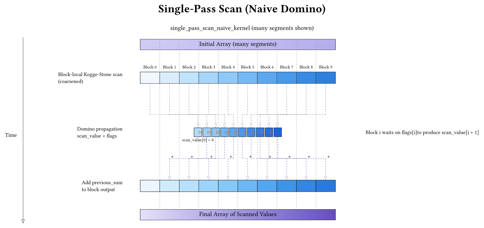
The domino chain needs two pieces of global state:
- Published prefixes: a per-block slot where block \(i\) publishes the prefix up to the end of its tile, so block \(i+1\) can read it.
- Readiness markers: a per-block marker so the successor knows the published prefix is valid and globally visible.
In the code these are scan_value (the published prefix values) and flags (the readiness markers). The epoch value is a generation counter: instead of clearing flags between invocations, the kernel treats flags[k] == epoch as “ready for this run”.
One small indexing convenience shows up in the snippet below: the arrays are effectively shifted by one (bid + 1) so slot 0 can represent the empty prefix (0). Block bid publishes into slot bid+1 and waits on slot bid.
The publish sequence requires a global memory fence:
scan_value[bid + 1] = previous_sum + block_sum;
__threadfence();
atomicExch(&flags[bid + 1], epoch);
Why __threadfence()? Because __syncthreads() only synchronizes threads inside a block. We need to ensure that block i’s write to scan_value[i+1] is globally visible before block i+1 observes flags[i+1] and proceeds. Without the fence, the successor block could read stale data.
Naive ordering hazard: these kernels use blockIdx.x as the logical block id. If CUDA schedules blocks out of order (which is allowed), the domino chain can deadlock. Concretely, a later block can become resident and spin waiting for a predecessor that was never scheduled; if all resident blocks are waiting, no block makes progress. This is why the next variant exists.
Dynamic block indexing scan
Kernel: src/single_pass_scan_dynamic_block_index.cu
To make the domino chain follow actual execution order (instead of launch order), blocks take a ticket from a global counter when they start running. That ticket becomes the block’s logical id in the chain, so a block never waits on a predecessor that hasn’t been scheduled yet.
In code, thread 0 does:
if (threadIdx.x == 0) {
    bid_s = atomicAdd(blockCounter, 1);
}
Because tickets are handed out in arrival order, the predecessor of ticket \(k\) (ticket \(k-1\)) must already be resident (it had to run to take ticket \(k-1\)), so the wait cannot be on a non-resident block. The rest of the logic (published prefixes, readiness flags, and __threadfence()) remains the same.
This approach is still a strict chain: every block still waits for its predecessor, but the ordering is now safe.
Decoupled lookbacks (single-pass)
Kernels:
Decoupled lookback removes the strict block-serialization of the domino chain. Terminology: I’ll call each block’s contiguous chunk of the input a tile. The algorithm maintains a global per-tile state array (called tile_state in the code) where each tile publishes information that later tiles can reuse.
Instead of “wait only for your immediate predecessor”, each tile:
- Publishes its local tile sum as a partial value in the tile-state array.
- Looks back over preceding tiles until it finds an inclusive tile, accumulating partial sums along the way.
- Publishes its own inclusive value (prefix + tile sum).
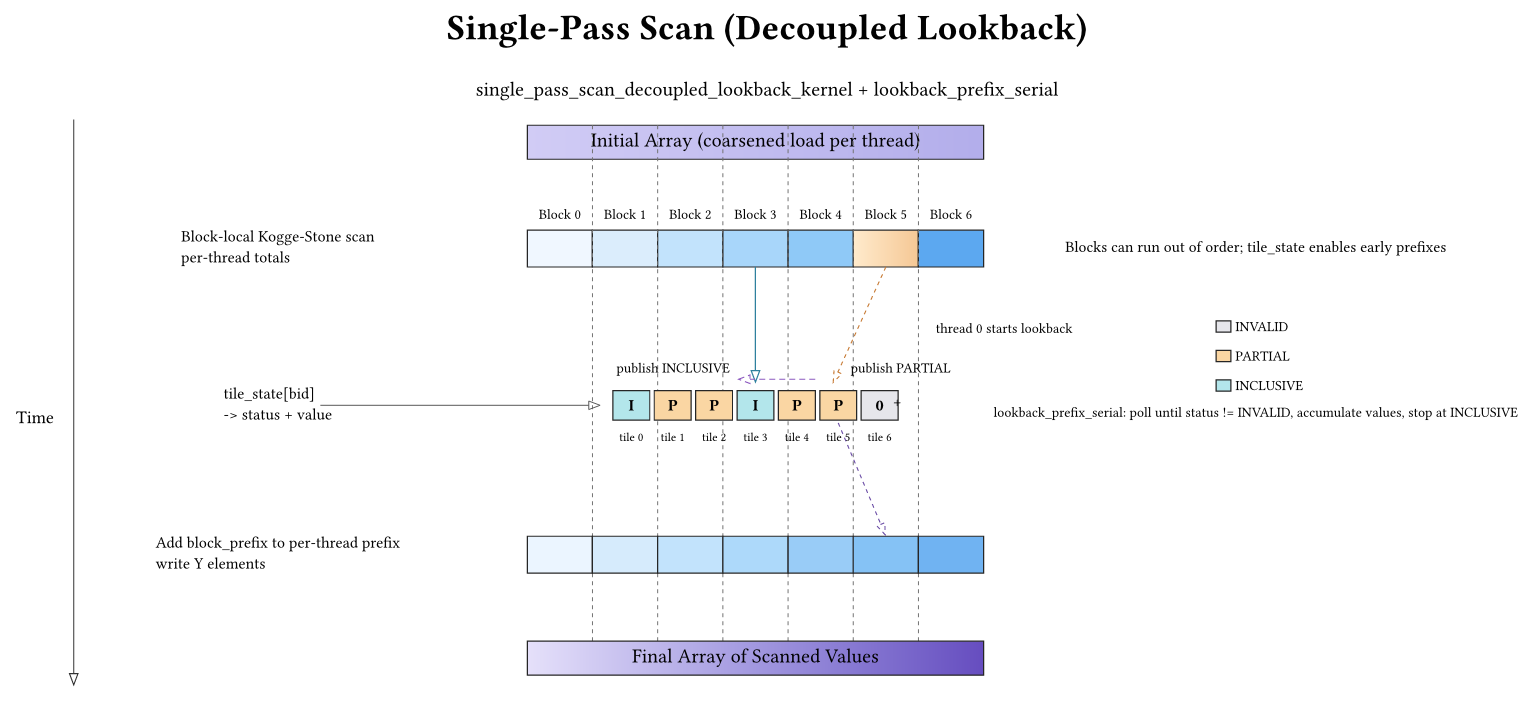
Tile state packing
Each tile state stores (status, value). Status is one of:
- Invalid (nothing published yet) —
TILE_INVALIDin the code - Partial (tile sum published; no carry from predecessors yet) —
TILE_PARTIALin the code - Inclusive (full prefix up to the end of the tile published) —
TILE_INCLUSIVEin the code
The code packs (status, value) into a single 64-bit word so updates can be atomic:
unsigned long long pack_state(unsigned int status, T value) {
    return (static_cast<unsigned long long>(status) << 32)
           | static_cast<unsigned long long>(__float_as_uint(static_cast<float>(value)));
}
This uses __float_as_uint and __uint_as_float to preserve the exact 32-bit bit pattern. The implementation assumes 32-bit values (sizeof(T) == sizeof(unsigned int)), which is enforced by a static_assert. If you want a type-safe version for non-float data, you would use a different packing strategy.
The lookback needs an atomic snapshot read of this 64-bit word. The code uses the CUDA idiom atomicAdd(&tile_state[idx], 0ULL) (atomic add of zero) as an atomic load, which ensures you see the most recent tile update while other blocks are publishing.
Serial lookback
Thread 0 walks backward until it sees an inclusive tile:
while (idx >= 0) {
    packed = atomicAdd(&tile_state[idx], 0ULL);
    unpack_state(packed, status, value);
    if (status != TILE_INVALID) {
        running += value;
        if (status == TILE_INCLUSIVE) { break; }
        idx -= 1;
    }
}
This lets blocks make progress even if predecessors have only published partial sums.
Warp-window lookback
The warp-window variant accelerates lookback by reading 32 tiles per iteration using a warp. Each lane reads one tile, the warp performs a prefix scan over that 32-tile window, and if any lane sees an INCLUSIVE tile the warp can stop immediately with the correct prefix.
T prefix = value;
for (int offset = 1; offset < WARP_SIZE; offset <<= 1) {
    T shifted = __shfl_up_sync(full_mask, prefix, offset);
    if (lane >= offset) { prefix += shifted; }
}

unsigned int inclusive_mask = __ballot_sync(full_mask, status == TILE_INCLUSIVE);
if (inclusive_mask) {
    int first = __ffs(inclusive_mask) - 1;
    T inclusive_prefix = __shfl_sync(full_mask, prefix, first);
    if (lane == 0) { running += inclusive_prefix; }
}
This reduces global memory polling by a factor of ~32 compared to the serial lookback.
The logic is subtle but important: the warp-level prefix scan computes cumulative sums over a 32-tile window. If any lane sees an INCLUSIVE tile, the prefix at that lane already includes all partials between the current block and that inclusive tile, so it is the correct prefix for the block. If no inclusive tile exists in the window, the warp adds the sum of the entire window and moves the lookback back by 32 tiles—no double counting because windows do not overlap.
How this differs from dynamic block indexing
- Dynamic block indexing still enforces a strict chain (block i waits for block i-1).
- Decoupled lookback lets blocks make partial progress even if predecessors are not finished, which improves parallelism when many blocks are resident.
- State footprint: lookback uses one packed per-tile state array (named
tile_statein the code). The dynamic-index domino uses a published-prefix array + readiness flags + a global ticket counter (namedscan_value,flags,blockCounter).
Performance Overview (from the provided benchmarks)
The repository includes benchmark results in bench/timing.txt, generated by running bench.sh over all kernels and a set of input sizes. The benchmarks were run on an NVIDIA H100 GPU. These numbers are wall-clock kernel times reported by each binary.
Notes on reading the numbers:
- All times are in milliseconds and represent a single kernel’s timing output for the given N.
- Small-N results are dominated by launch/synchronization overheads; large-N results better reflect algorithmic scaling and memory behavior.
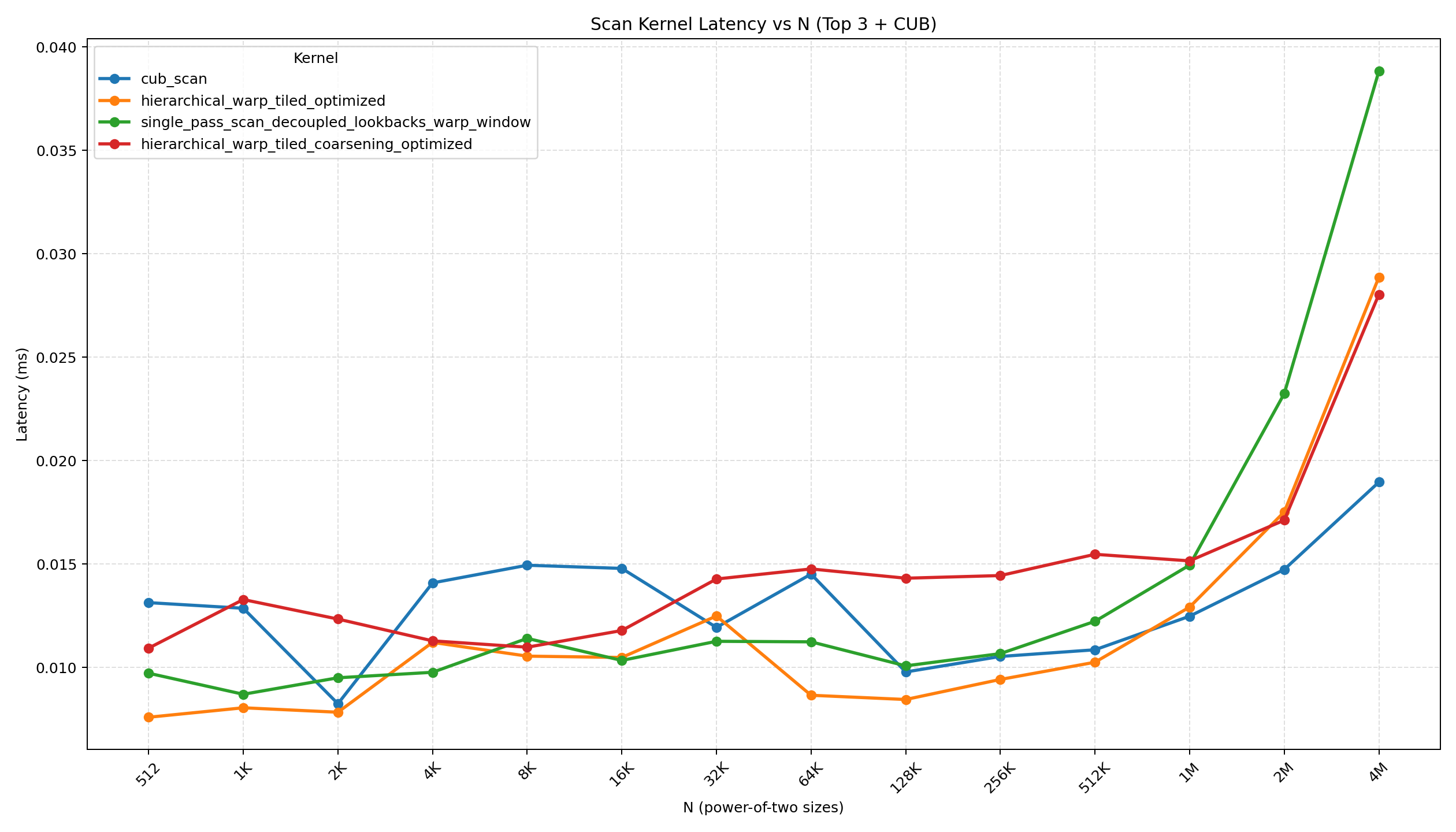
Latency plot (power-of-two sizes)
The plot below visualizes the top 3 kernels (by average power-of-two latency) plus CUB across power-of-two input sizes. It is generated from bench/timing.txt and saved at bench/latency_pow2_top3.png.
Small‑N snapshot (power‑of‑two sizes)
For very small inputs, fixed overheads (kernel launch, synchronization, and setup) dominate. The absolute differences are tiny, but it’s still useful to see which kernels stay competitive when N is small.
| Kernel (selected) | N = 512 (ms) | N = 1,024 (ms) | N = 2,048 (ms) | N = 4,096 (ms) | N = 8,192 (ms) |
|---|---|---|---|---|---|
| CUB DeviceScan | 0.013136 | 0.012864 | 0.0082496 | 0.0140896 | 0.014944 |
| Hierarchical warp-tiled optimized | 0.0075968 | 0.0080544 | 0.00784 | 0.011216 | 0.0105504 |
| Single-pass decoupled lookback (warp window) | 0.0097248 | 0.0087072 | 0.009504 | 0.0097696 | 0.011408 |
| Hierarchical warp-tiled coarsened optimized | 0.0109376 | 0.0132864 | 0.0123424 | 0.0112896 | 0.0109824 |
Observations (small N):
- Differences are within a few microseconds, so launch and synchronization overheads dominate.
- The warp-tiled optimized variant is consistently strong, suggesting its low sync count helps even at small N.
- The coarsened optimized variant carries extra shared-memory traffic and setup, which can be less favorable at tiny sizes.
Large‑N snapshot (representative sizes)
Below is a snapshot of representative larger sizes from bench/timing.txt. (Lower is better.)
| Kernel (selected) | N = 100,000 (ms) | N = 1,000,000 (ms) | N = 4,194,303 (ms) |
|---|---|---|---|
| CUB DeviceScan | 0.0139072 | 0.0121504 | 0.0190912 |
| Hierarchical Kogge-Stone | 0.0101056 | 0.0189024 | 0.0597216 |
| Hierarchical Kogge-Stone (double buffer) | 0.0109184 | 0.0179616 | 0.0564128 |
| Hierarchical Brent-Kung | 0.0131008 | 0.0216928 | 0.0584768 |
| Hierarchical warp-tiled optimized | 0.0110592 | 0.0128512 | 0.02824 |
| Hierarchical warp-tiled coarsened optimized | 0.0141440 | 0.0156544 | 0.0278208 |
| Single-pass decoupled lookback | 0.0128544 | 0.0213984 | 0.0563424 |
| Single-pass decoupled lookback (warp window) | 0.01008 | 0.014992 | 0.0386688 |
| Single-pass dynamic block index | 0.029392 | 0.230454 | 0.946202 |
| Single-pass naive | 0.0302944 | 0.221734 | 0.910448 |
Takeaways
- Warp-tiled hierarchical scans are consistently strong at large N. They combine coalesced access with warp primitives and fewer synchronization points, so they stay competitive as the array grows.
- CUB is a strong baseline, often among the fastest (as expected).
- Decoupled lookback with warp-window usually beats the serial lookback because the warp cooperatively scans 32 tiles at a time, reducing the number of global polls.
- Naive and dynamic-block-index single-pass scans degrade at large N. The domino chain introduces strong serialization, which dominates as the number of blocks grows.
- Brent-Kung double buffering does not help in these measurements, matching the reasoning in the notes: the in-place Brent-Kung already avoids the hazards that double buffering tries to fix.
If you want to reproduce or extend these results, bench.sh runs all binaries under bin/ and prints the same table format used in bench/timing.txt.
Conclusion
- Hierarchical scans provide a clear, scalable baseline with predictable synchronization.
- Coarsening and double buffering highlight memory and synchronization tradeoffs.
- Warp-tiled optimizations show how warp primitives and register tiling reduce shared-memory pressure and synchronization overhead.
- Single-pass scans demonstrate how to coordinate blocks without global barriers, from simple dominos to sophisticated decoupled lookbacks.
If you are new to GPU scans, start with the simple hierarchical Kogge-Stone and Brent-Kung versions and study how the block-totals buffer enables global correctness. Then move to the coarsened and warp-tiled kernels to see how memory coalescing and warp primitives change the design. Finally, explore single-pass scans to understand how inter-block coordination can be done without extra kernel launches.