Paper Summary #15 - Hyper-Connections and mHC
Papers: Hyper-Connections and mHC: Manifold-Constrained Hyper-Connections
Residual product growth
Small per-layer gains compound quickly when the residual path is a learned multiplier chain.
Sinkhorn normalization
Column and row normalization push a positive matrix toward the doubly stochastic constraint.
Hyper-Connections (HC) generalize the residual stream into multiple learned streams. Manifold-Constrained Hyper-Connections (mHC) keep that extra routing capacity while constraining the residual mixing matrices so deep products remain stable.
The baseline: what residual connections are really buying us
A standard residual layer is:
\[\mathbf{x}_{l+1} = \mathbf{x}_l + \mathcal{F}(\mathbf{x}_l, \mathcal{W}_l),\]where:
- $\mathbf{x}_l \in \mathbb{R}^{C}$ is the residual-stream state at layer $l$,
- $\mathcal{F}$ is the layer body, e.g. attention or MLP,
- $\mathcal{W}_l$ are the layer weights.
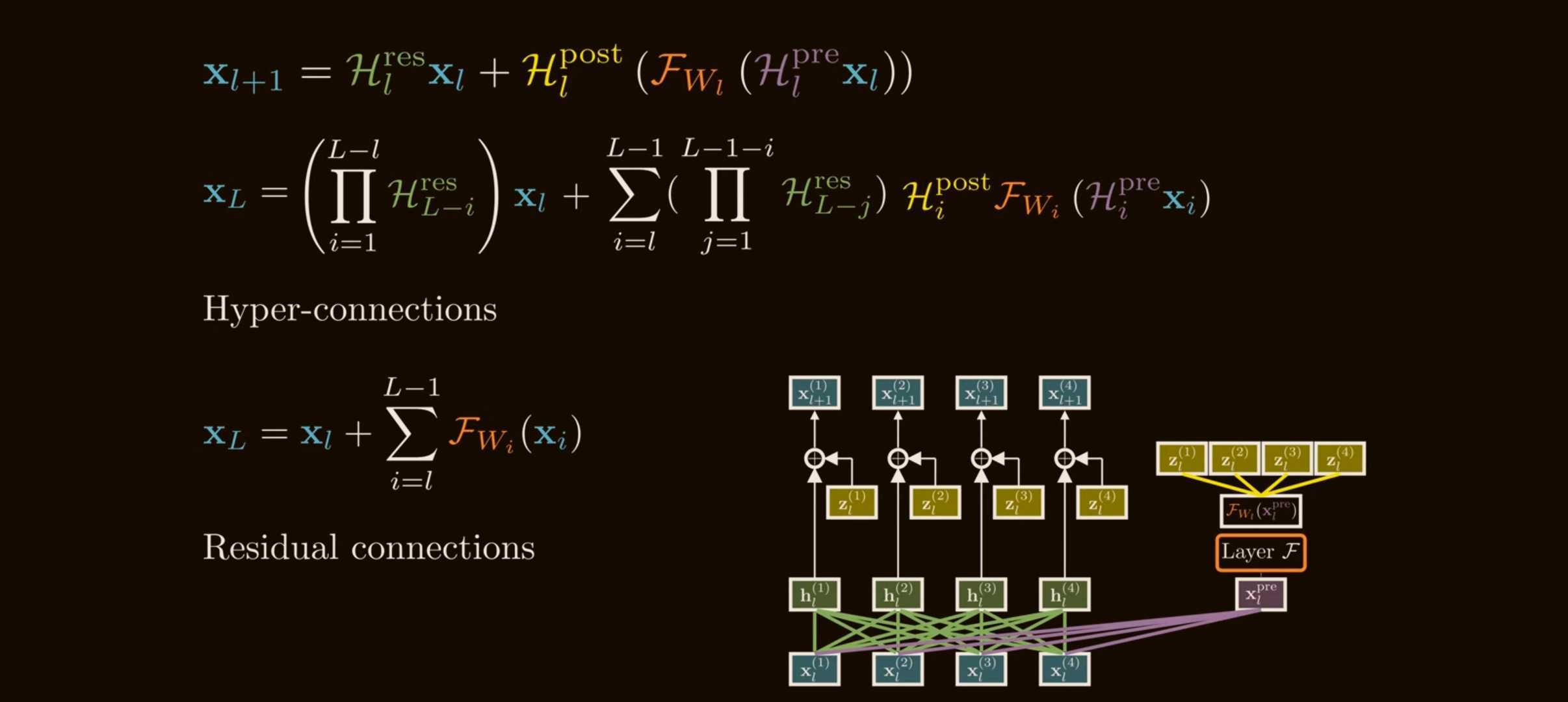
The important part is not just the addition. It is the identity path. If we recursively expand from a shallow layer $l$ to a deeper layer $L$, we get:
\[\mathbf{x}_L = \mathbf{x}_l + \sum_{i=l}^{L-1}\mathcal{F}(\mathbf{x}_i,\mathcal{W}_i).\]The shallow signal $\mathbf{x}_l$ reaches layer $L$ unchanged. This gives deep networks a stable highway for forward activations and backward gradients.
Why this matters:
- without a skip path, deep networks must repeatedly multiply through learned transformations, so signals can vanish or explode;
- with the identity path, the model can start near a shallow network and learn residual corrections;
- in Transformers, the residual stream is the persistent memory channel through which attention and MLP blocks communicate.
The classical residual connection is stable, but rigid. Every layer receives exactly one stream and writes back to exactly one stream.
The problem HC was trying to solve
Residual variants such as Pre-Norm and Post-Norm make a trade-off:
- Pre-Norm stabilizes gradients, but can make adjacent deep representations overly similar. This is the “representation collapse” side of the trade-off.
- Post-Norm can improve representational separation, but is more prone to gradient vanishing.
The HC paper frames this as a “seesaw”: fixed residual wiring chooses one point on the stability-vs-expressivity curve. Hyper-Connections ask: can the network learn how strongly layers should connect, instead of hard-coding the residual topology?
The key HC move is to widen the residual stream.
Instead of carrying one vector:
\[\mathbf{x}_l \in \mathbb{R}^{C},\]HC carries $n$ parallel residual streams:
\[\mathbf{x}_l = \begin{bmatrix} \mathbf{x}_{l,0} \\ \mathbf{x}_{l,1} \\ \vdots \\ \mathbf{x}_{l,n-1} \end{bmatrix} \in \mathbb{R}^{n \times C}.\]Here $n$ is the expansion rate. In the DeepSeek mHC paper, experiments commonly use $n=4$.
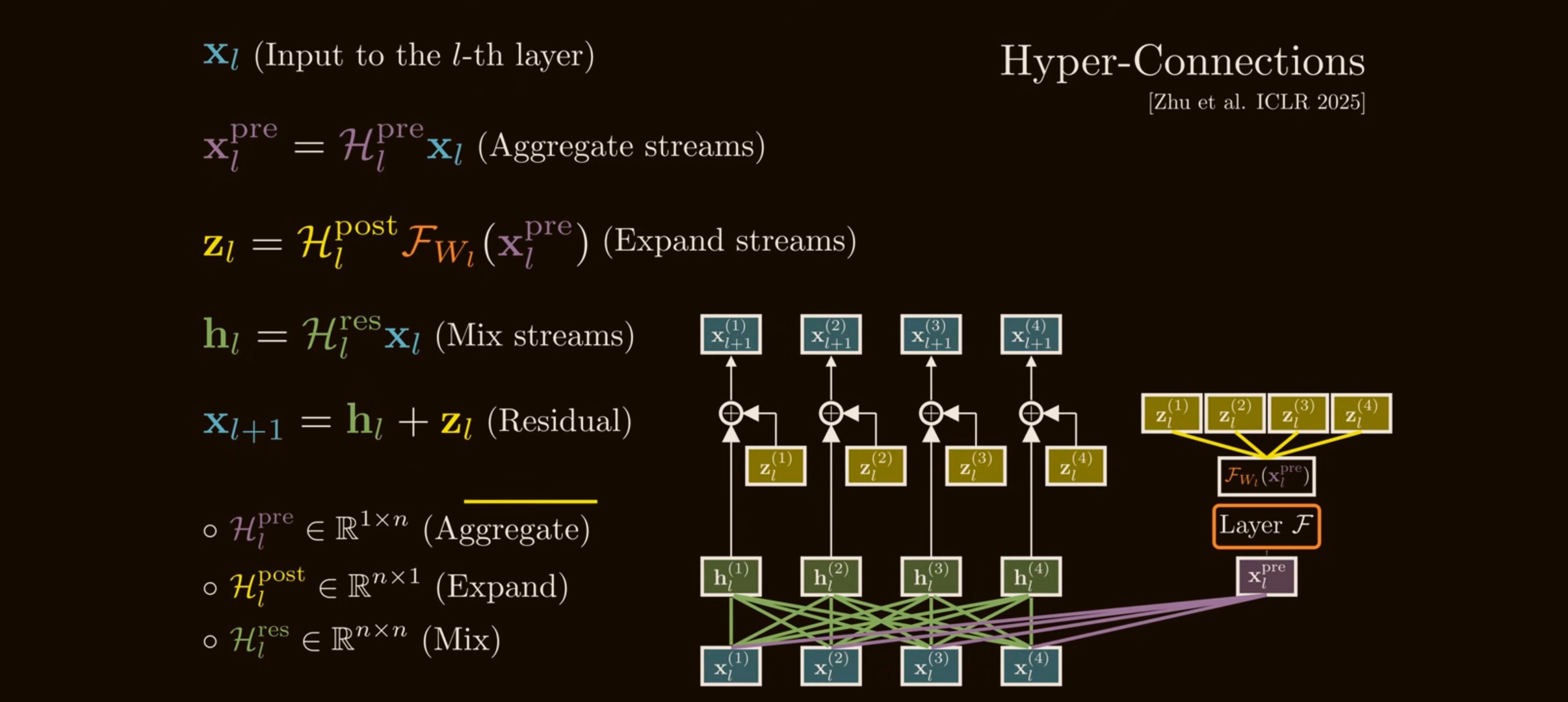
The layer body $\mathcal{F}$ still expects a normal $C$-dimensional input, so HC needs three maps:
- Pre / aggregation map $\mathcal{H}_l^{\mathrm{pre}} \in \mathbb{R}^{1 \times n}$: combines $n$ streams into one layer input.
- Post / expansion map $\mathcal{H}_l^{\mathrm{post}} \in \mathbb{R}^{1 \times n}$: writes the layer output back into $n$ streams.
- Residual mixing map $\mathcal{H}_l^{\mathrm{res}} \in \mathbb{R}^{n \times n}$: mixes the residual streams directly.
The single-layer HC update is:
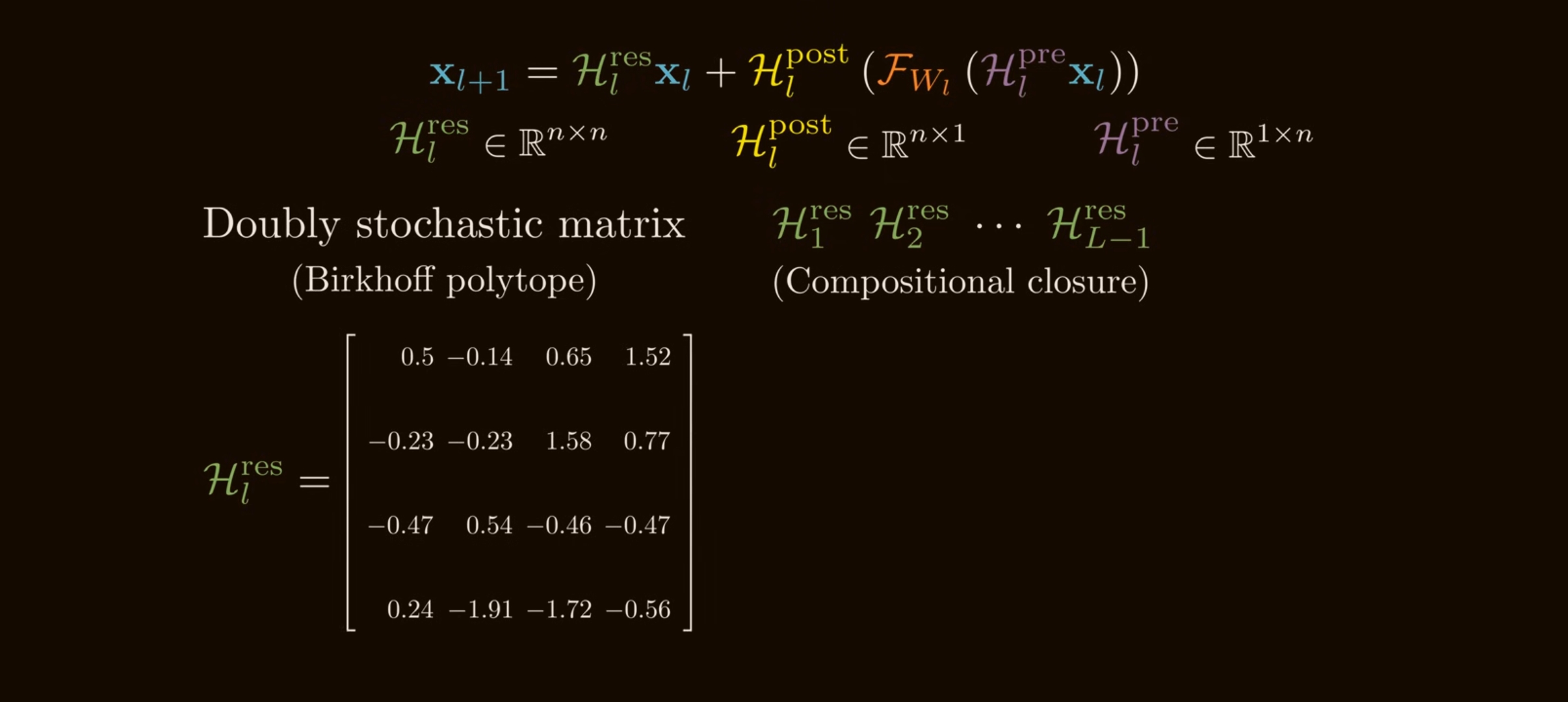
\[\mathbf{x}_{l+1} = \mathcal{H}_{l}^{\mathrm{res}}\mathbf{x}_l + \mathcal{H}_{l}^{\mathrm{post}\,\top} \mathcal{F}\left( \mathcal{H}_{l}^{\mathrm{pre}}\mathbf{x}_l, \mathcal{W}_l \right).\]This is the same residual idea, but generalized:
- $\mathcal{H}_l^{\mathrm{pre}}\mathbf{x}_l$ chooses what mixture of streams enters attention or MLP;
- $\mathcal{H}_l^{\mathrm{post}\,\top}\mathcal{F}(\cdot)$ chooses where the new layer output is written;
- $\mathcal{H}_l^{\mathrm{res}}\mathbf{x}_l$ lets old streams exchange information before the new residual update is added.
In implementation terms, a single HC residual layer looks like this:
def hyper_connection_layer(x, layer_fn, h_pre, h_post, h_res):
    """
    x:      [n, C] multi-stream residual state
    h_pre:  [n]    aggregates streams into one layer input
    h_post: [n]    writes layer output back to streams
    h_res:  [n, n] mixes streams directly
    """
    layer_input = h_pre @ x                 # [C]
    layer_output = layer_fn(layer_input)    # [C]
    residual_mix = h_res @ x                # [n, C]
    write_back = h_post[:, None] * layer_output[None, :]
    return residual_mix + write_back
Original HC notation: depth and width connections
The original Hyper-Connections paper writes the connection matrix as:
\[\mathcal{HC} = \begin{pmatrix} \mathbf{0}_{1\times1} & \mathbf{B} \\ \mathbf{A}_m & \mathbf{A}_r \end{pmatrix} \in \mathbb{R}^{(n+1)\times(n+1)}.\]For a network layer $\mathcal{T}$ and hyper-hidden matrix $\mathbf{H}\in\mathbb{R}^{n\times d}$:
\[\hat{\mathbf{H}} = \mathbf{B}^{\top}\mathcal{T}(\mathbf{H}^{\top}\mathbf{A}_m)^{\top} + \mathbf{A}_r^{\top}\mathbf{H}.\]Mapping this to the mHC notation:
| Original HC paper | mHC paper notation | Role |
|---|---|---|
| $\mathbf{A}_m$ | $\mathcal{H}^{\mathrm{pre}}$ | aggregate $n$ streams into layer input |
| $\mathbf{B}$ | $\mathcal{H}^{\mathrm{post}}$ | write layer output back to streams |
| $\mathbf{A}_r$ | $\mathcal{H}^{\mathrm{res}}$ | residual-stream mixing |
HC further decomposes this into:
\[\mathcal{DC} = \begin{pmatrix} \mathbf{B}\\ \mathrm{diag}(\mathbf{A}_r) \end{pmatrix}, \qquad \mathcal{WC} = \begin{pmatrix} \mathbf{A}_m & \mathbf{A}_r \end{pmatrix}.\]The intuition:
- depth-connections learn how much each stream should preserve old information versus accept new layer output;
- width-connections learn how streams communicate laterally at the same depth.
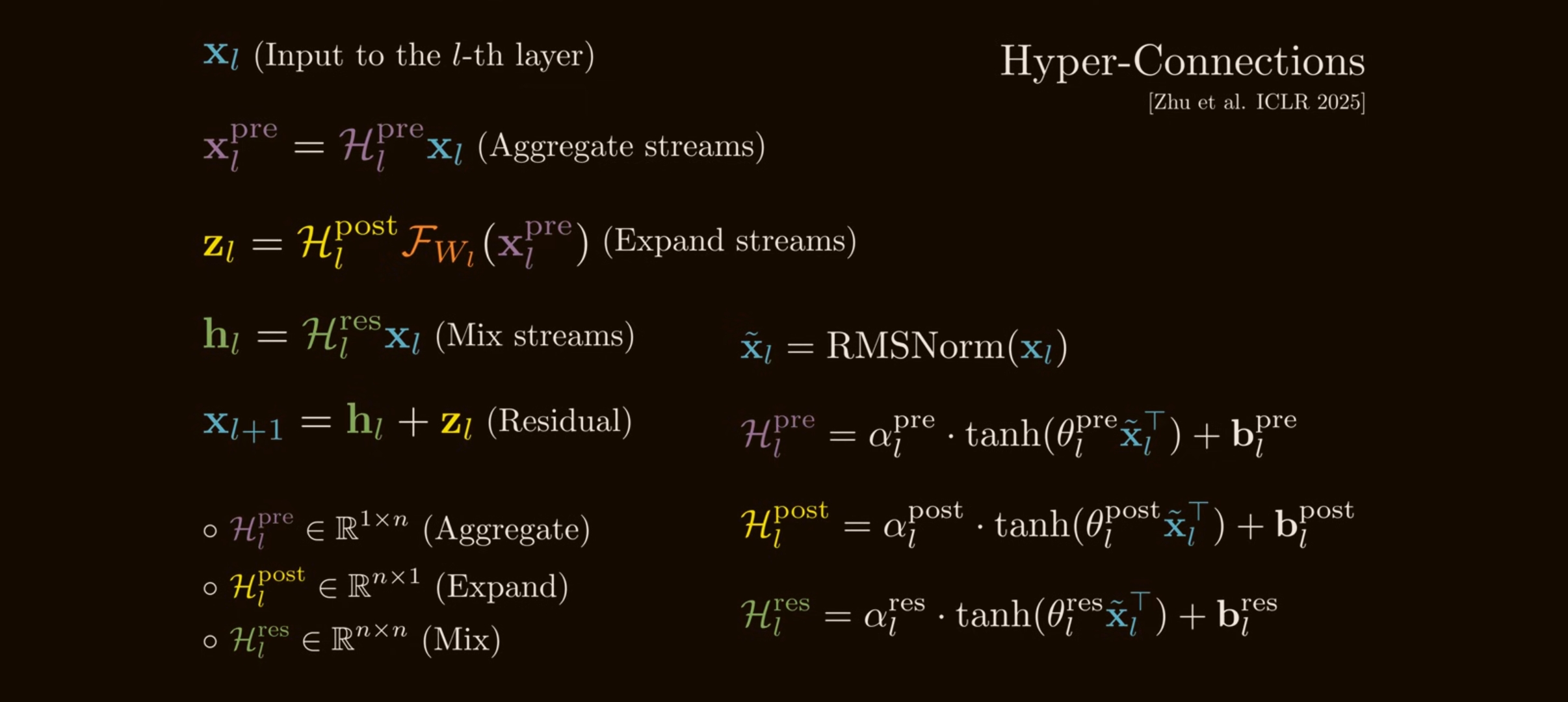
The original HC paper also introduces dynamic Hyper-Connections, where the maps are input-conditioned:
\[\overline{\mathbf{H}}=\mathrm{norm}(\mathbf{H}),\] \[\mathcal{B}(\mathbf{H}) = s_\beta \circ \tanh(\overline{\mathbf{H}}\mathbf{W}_\beta)^\top + \mathbf{B},\] \[\mathcal{A}_m(\mathbf{H}) = s_\alpha \circ \tanh(\overline{\mathbf{H}}\mathbf{W}_m) + \mathbf{A}_m,\] \[\mathcal{A}_r(\mathbf{H}) = s_\alpha \circ \tanh(\overline{\mathbf{H}}\mathbf{W}_r) + \mathbf{A}_r.\]The small learned gates $s_\alpha,s_\beta$ keep the dynamic part small at initialization. In the original paper, dynamic HC with expansion $n=4$ was especially useful in language-model pretraining and achieved much faster convergence in the OLMoE setting.
Why HC can improve models
HC increases macro-architectural flexibility without making attention or MLP blocks wider.
That is the important scaling argument:
- increasing $C$ makes attention projections and MLPs much more expensive;
- increasing $n$ adds multiple residual streams, but the layer body still sees a $C$-dimensional vector;
- since typical $n$ is small, e.g. $n=4$, the extra coefficient maps are much cheaper than the block itself.
Conceptually, HC gives the model a learned routing topology across depth.
Special cases:
- if the maps are chosen one way, HC behaves like a standard sequential residual network;
- if chosen another way, it can emulate parallel transformer blocks;
- with dynamic maps, different tokens can use different soft layer arrangements.
This is why the HC paper argues that Hyper-Connections can learn mixtures of Pre-Norm-like, Post-Norm-like, sequential, and parallel wiring.
The instability: products of residual mixing matrices
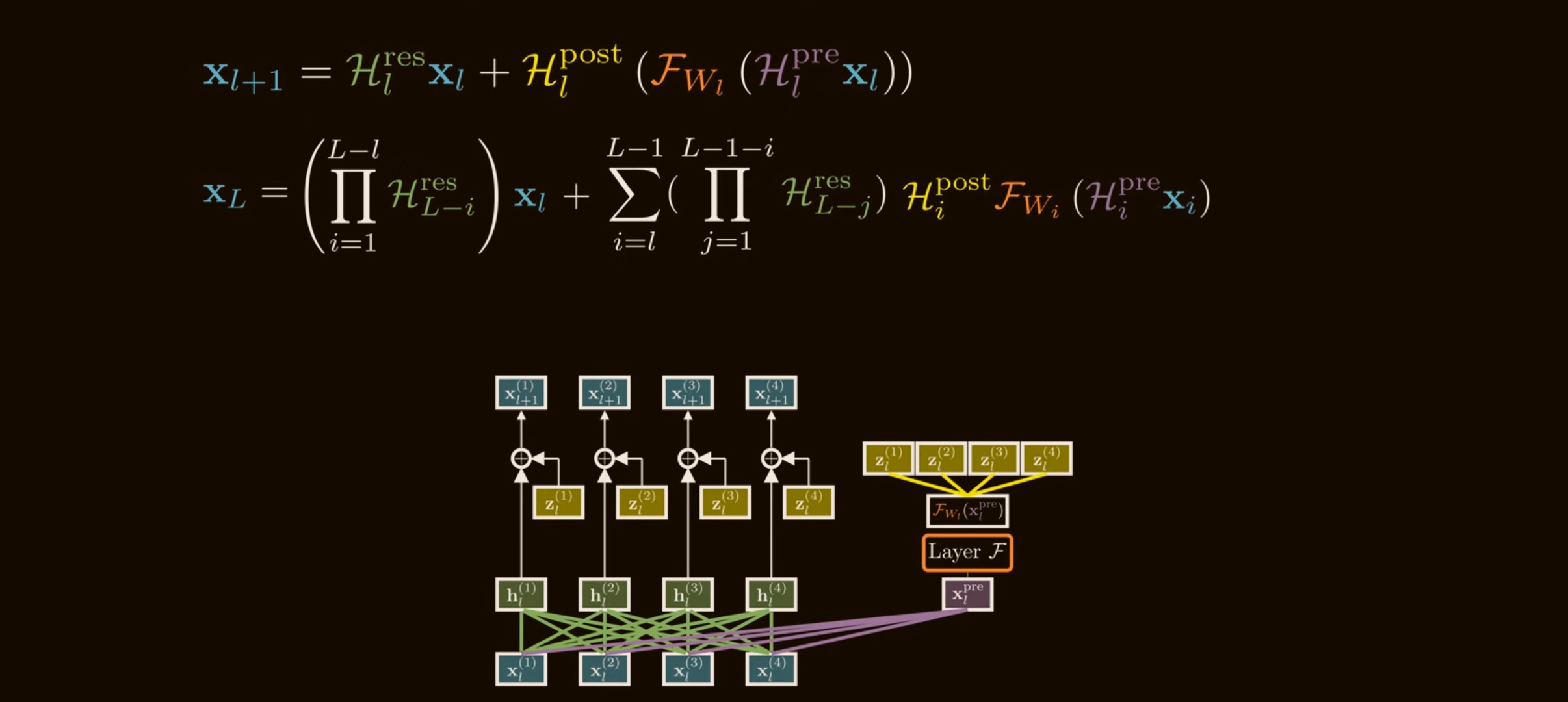
The problem appears when we stack many HC layers. Expanding the single-layer update over depth gives:
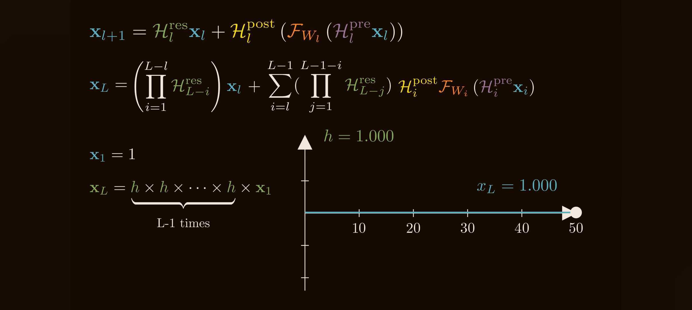
\[\mathbf{x}_{L} = \left( \prod_{i=1}^{L-l} \mathcal{H}_{L-i}^{\mathrm{res}} \right)\mathbf{x}_l + \sum_{i=l}^{L-1} \left( \prod_{j=1}^{L-1-i} \mathcal{H}_{L-j}^{\mathrm{res}} \right) \mathcal{H}_{i}^{\mathrm{post}\,\top} \mathcal{F}( \mathcal{H}_{i}^{\mathrm{pre}}\mathbf{x}_i, \mathcal{W}_i).\]This has two pieces:
- The shallow feature $\mathbf{x}_l$ transformed by a product of residual mixing matrices.
- A sum of every previous layer output, each also transformed by products of later residual mixing matrices.
With a standard residual connection, the shallow feature path is just $\mathbf{x}_l$. With HC, it is:
\[\left( \mathcal{H}_{L-1}^{\mathrm{res}} \mathcal{H}_{L-2}^{\mathrm{res}} \cdots \mathcal{H}_{l}^{\mathrm{res}} \right)\mathbf{x}_l.\]That product is the danger.
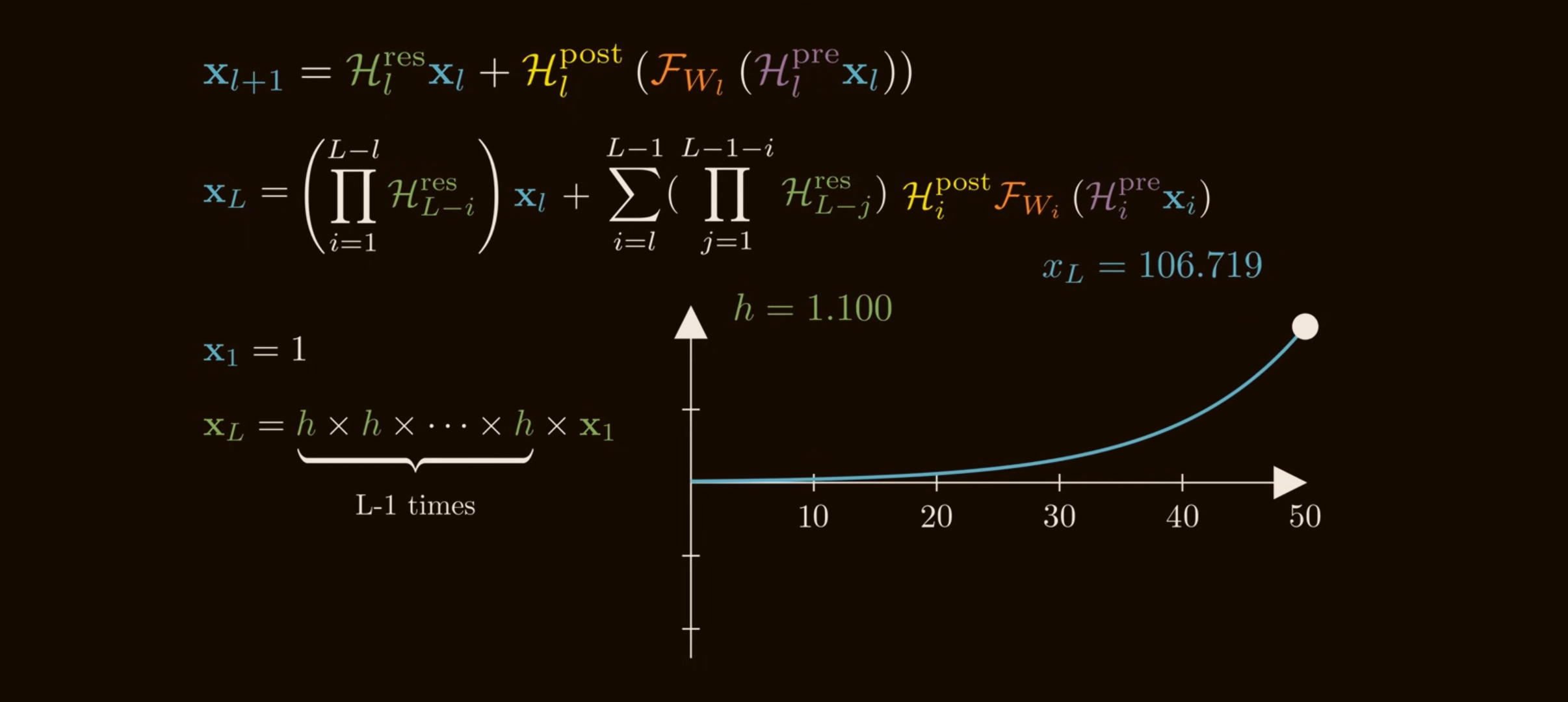
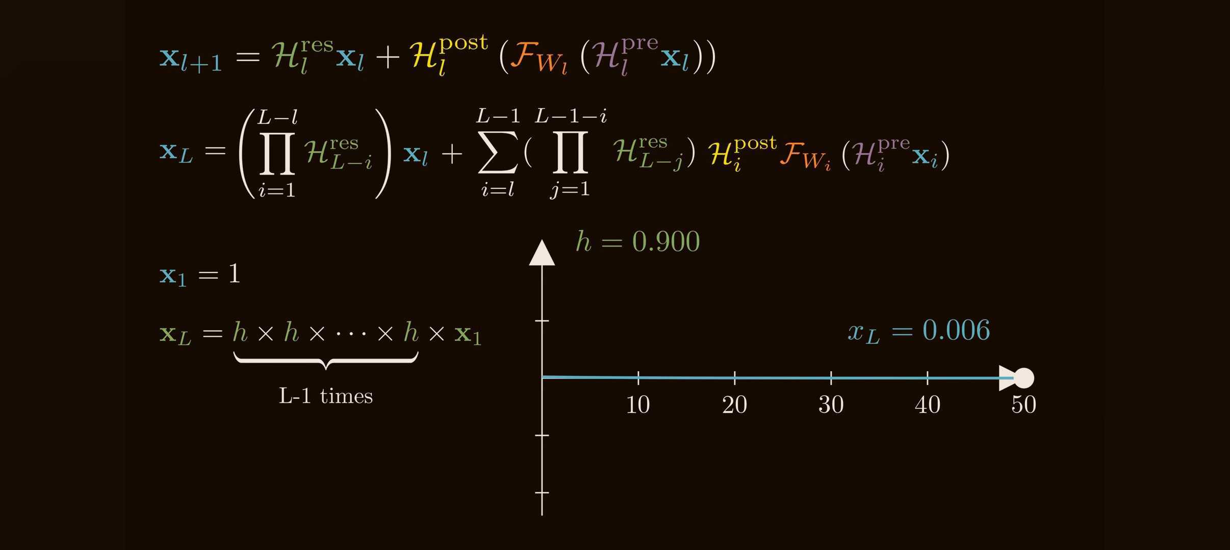
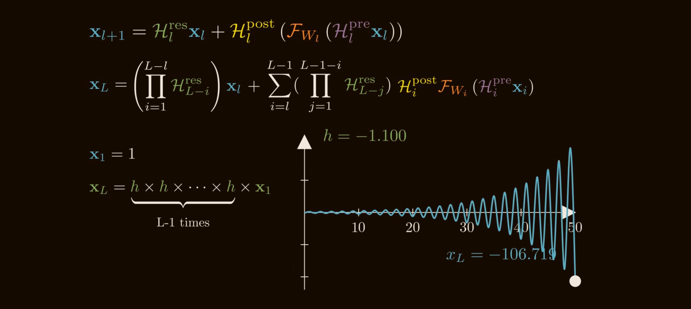
If each $\mathcal{H}_l^{\mathrm{res}}$ is unconstrained, even small deviations from identity compound. A simple scalar analogy shows the issue:
\[1.05^{100}\approx 131.5, \qquad 0.95^{100}\approx 0.0059.\]Tiny per-layer amplification becomes explosion; tiny per-layer attenuation becomes disappearance. Matrices are worse because different directions can amplify or shrink differently.
The mHC paper measures this using Amax Gain Magnitude:
\[G_{\mathrm{fwd}}(M) = \max_i\left|\sum_j M_{ij}\right|,\] \[G_{\mathrm{bwd}}(M) = \max_j\left|\sum_i M_{ij}\right|.\]For a composite residual map:
\[M_{l\to L} = \prod_{i=1}^{L-l}\mathcal{H}_{L-i}^{\mathrm{res}},\]$G_{\mathrm{fwd}}$ captures worst-case forward signal gain, and $G_{\mathrm{bwd}}$ captures worst-case backward gradient gain.
DeepSeek reports that HC can hit Amax gain values near $3000$ in 27B-scale experiments. That is no longer a gentle residual highway; it is a learned multiplier chain.
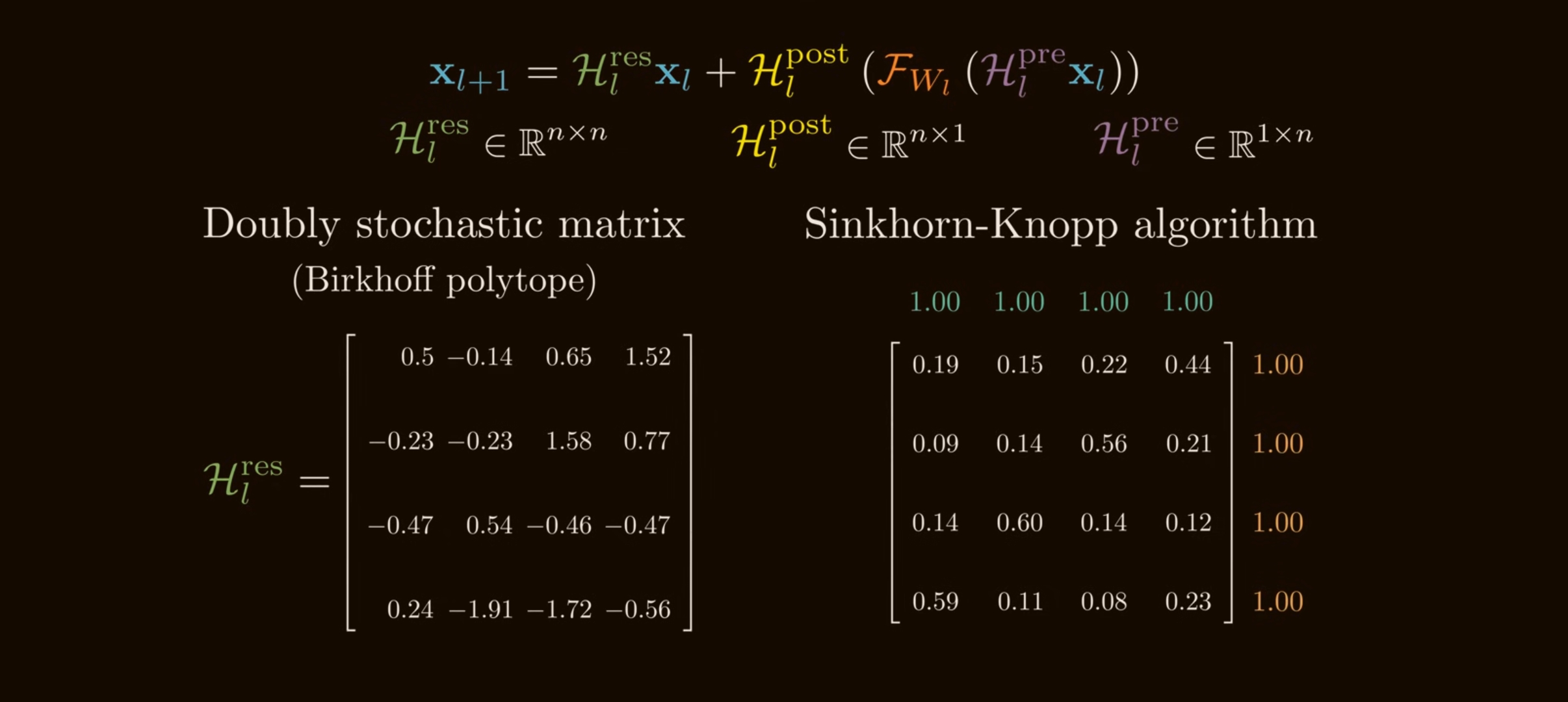
mHC’s core fix: constrain residual mixing to the Birkhoff polytope
mHC keeps the useful part of HC: multiple residual streams and learned stream mixing.
But it constrains the residual mixing matrix:
\[\mathcal{H}_{l}^{\mathrm{res}} \in \mathcal{M}^{\mathrm{res}},\]where:
\[\mathcal{M}^{\mathrm{res}} = \left\{ H\in\mathbb{R}^{n\times n} \mid H\mathbf{1}_n=\mathbf{1}_n,\; \mathbf{1}_n^\top H=\mathbf{1}_n^\top,\; H\ge 0 \right\}.\]This is the set of doubly stochastic matrices, also called the Birkhoff polytope.
A matrix is doubly stochastic if:
- all entries are non-negative;
- every row sums to $1$;
- every column sums to $1$.
Example:
\[H = \begin{bmatrix} 0.7 & 0.3\\ 0.3 & 0.7 \end{bmatrix}\]is doubly stochastic. It mixes the two streams, but it cannot create or delete average mass.
Why doubly stochastic matrices stabilize depth
There are three important properties.
They preserve the all-ones direction
If $H\mathbf{1}=\mathbf{1}$, each row sums to $1$. If $\mathbf{1}^\top H=\mathbf{1}^\top$, each column sums to $1$.
So $H$ acts like a conservative mixing operator over streams. It can redistribute signal among streams, but it cannot globally scale the stream average up or down.
They are non-expansive in spectral norm
For a non-negative doubly stochastic matrix:
\[\|H\|_1 = 1, \qquad \|H\|_\infty = 1.\]Using the norm inequality:
\[\|H\|_2 \le \sqrt{\|H\|_1\|H\|_\infty} =1.\]Therefore:
\[\|H\mathbf{x}\|_2 \le \|\mathbf{x}\|_2.\]This directly attacks gradient explosion through $\mathcal{H}^{\mathrm{res}}$.
They are closed under multiplication
If $A$ and $B$ are doubly stochastic, then $AB$ is also doubly stochastic:
\[AB\mathbf{1}=A(B\mathbf{1})=A\mathbf{1}=\mathbf{1},\] \[\mathbf{1}^\top AB=(\mathbf{1}^\top A)B=\mathbf{1}^\top B=\mathbf{1}^\top,\]and $AB\ge 0$ because $A,B\ge 0$.
This is the crucial depth property. The composite map:
\[M_{l\to L} = \prod_{i=1}^{L-l}\mathcal{H}_{L-i}^{\mathrm{res}}\]is also doubly stochastic if every factor is doubly stochastic. Stability survives depth.
Geometrically, the Birkhoff-von Neumann theorem says the Birkhoff polytope is the convex hull of permutation matrices:
\[H = \sum_{k} \lambda_k P_k, \qquad \lambda_k\ge 0, \qquad \sum_k \lambda_k=1.\]So mHC residual mixing is a soft mixture of stream permutations. It can route and combine streams, but within a conservative envelope.
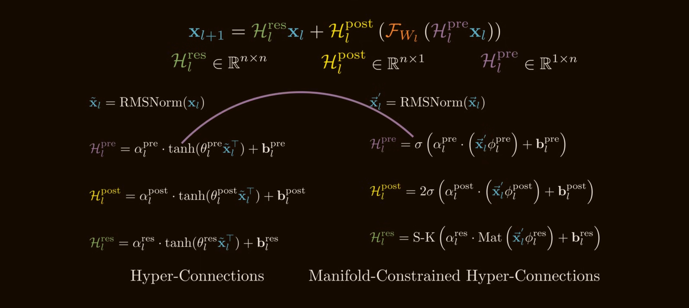
How mHC constructs the constrained maps
mHC first computes unconstrained pre-activations from the flattened $n$-stream state:
\[\vec{\mathbf{x}}_l = \mathrm{vec}(\mathbf{x}_l) \in \mathbb{R}^{1\times nC}.\]Then:
\[\begin{aligned} \vec{\mathbf{x}}'_l &= \mathrm{RMSNorm}(\vec{\mathbf{x}}_l), \\ \widetilde{\mathcal{H}}_l^{\mathrm{pre}} &= \alpha_l^{\mathrm{pre}} (\vec{\mathbf{x}}'_l\phi_l^{\mathrm{pre}}) +\mathbf{b}_l^{\mathrm{pre}}, \\ \widetilde{\mathcal{H}}_l^{\mathrm{post}} &= \alpha_l^{\mathrm{post}} (\vec{\mathbf{x}}'_l\phi_l^{\mathrm{post}}) +\mathbf{b}_l^{\mathrm{post}}, \\ \widetilde{\mathcal{H}}_l^{\mathrm{res}} &= \alpha_l^{\mathrm{res}} \mathrm{mat}(\vec{\mathbf{x}}'_l\phi_l^{\mathrm{res}}) +\mathbf{b}_l^{\mathrm{res}}. \end{aligned}\]The final constrained maps are:
\[\begin{aligned} \mathcal{H}_l^{\mathrm{pre}} &= \sigma(\widetilde{\mathcal{H}}_l^{\mathrm{pre}}), \\ \mathcal{H}_l^{\mathrm{post}} &= 2\sigma(\widetilde{\mathcal{H}}_l^{\mathrm{post}}), \\ \mathcal{H}_l^{\mathrm{res}} &= \mathrm{SinkhornKnopp} (\widetilde{\mathcal{H}}_l^{\mathrm{res}}). \end{aligned}\]Two details matter:
- sigmoid makes $\mathcal{H}^{\mathrm{pre}}$ and $\mathcal{H}^{\mathrm{post}}$ non-negative, reducing cancellation from positive/negative coefficient compositions;
- the factor $2$ on $\mathcal{H}^{\mathrm{post}}$ centers the post map around $1$ when its pre-activation is near zero, because $2\sigma(0)=1$ - making the hyper connections behave exactly like standard residual connections at the beginning of training.
Sinkhorn-Knopp: projecting to a doubly stochastic matrix
Given an unconstrained matrix $\widetilde{H}$, mHC first makes it positive:
\[M^{(0)} = \exp(\widetilde{H}).\]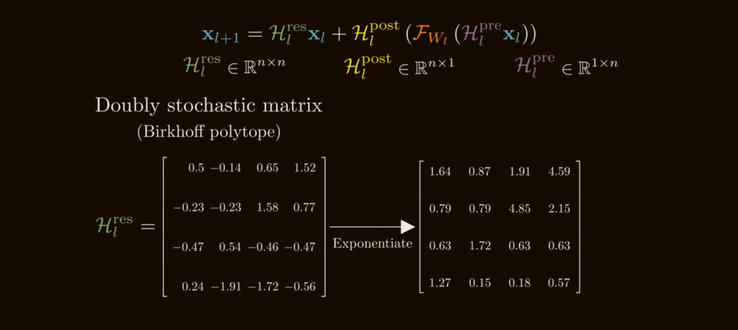
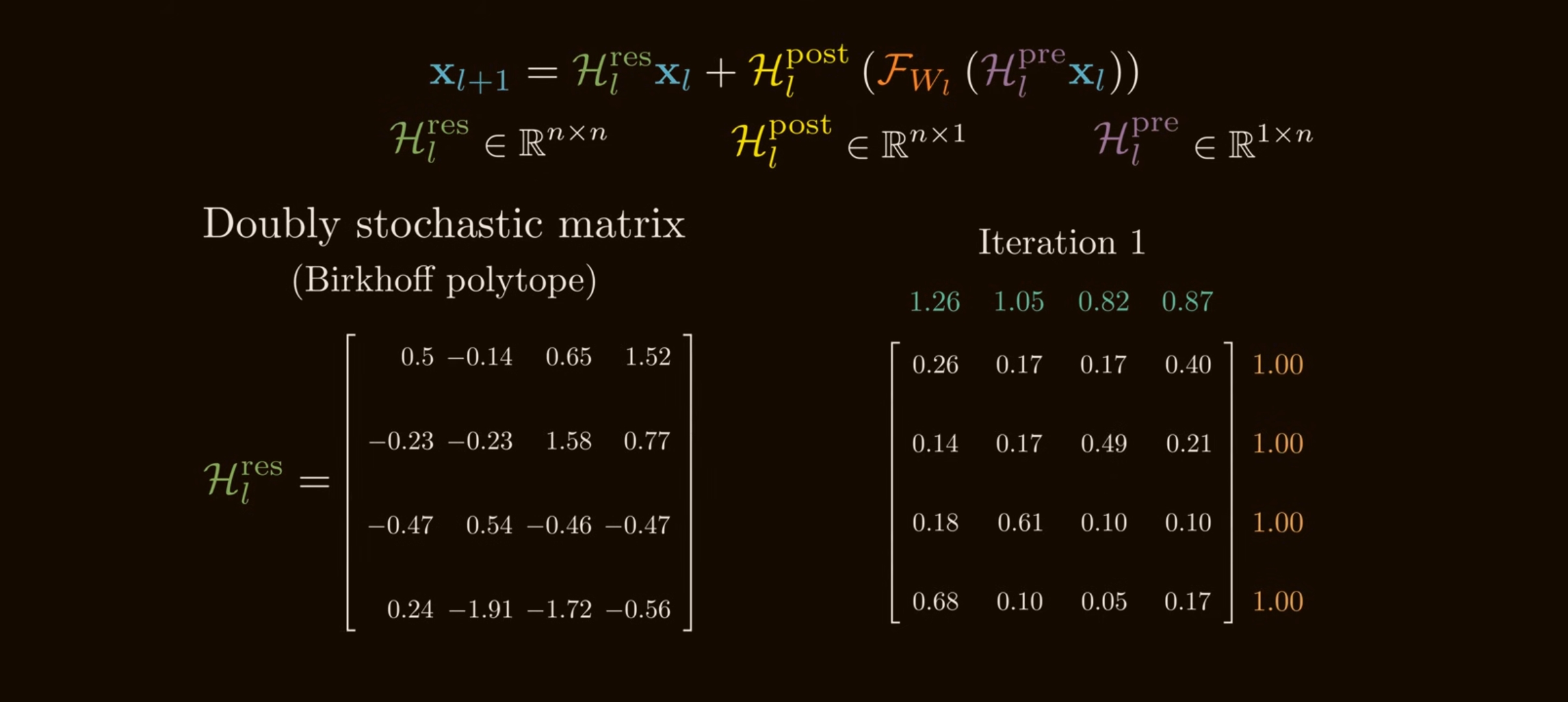
Then it alternates column and row normalization:
\[M^{(t)} = \mathcal{T}_r \left( \mathcal{T}_c(M^{(t-1)}) \right),\]where:
\[\mathcal{T}_c(M)_{ij} = \frac{M_{ij}}{\sum_{i'}M_{i'j}},\] \[\mathcal{T}_r(M)_{ij} = \frac{M_{ij}}{\sum_{j'}M_{ij'}}.\]Each column-normalization step fixes column sums. Each row-normalization step fixes row sums. Repeating the process converges toward a doubly stochastic matrix under standard positivity assumptions.
import numpy as np

def sinkhorn_knopp(logits, iters=20, eps=1e-12):
    """
    Project an unconstrained square matrix toward the Birkhoff polytope.

    logits: [n, n] unconstrained residual-mixing scores
    returns: approximately doubly stochastic [n, n] matrix
    """
    m = np.exp(logits)  # make entries positive

    for _ in range(iters):
        m = m / (m.sum(axis=0, keepdims=True) + eps)  # normalize columns
        m = m / (m.sum(axis=1, keepdims=True) + eps)  # normalize rows

    return m
In DeepSeek’s mHC experiments:
\[t_{\max}=20.\]Because finite iterations are approximate, mHC does not produce a mathematically exact doubly stochastic matrix in practice. But the paper reports that the composite Amax gain stays bounded around $1.6$, compared with nearly $3000$ for vanilla HC.
The full mHC update
Once the maps are constrained, the layer update keeps the HC form:
\[\mathbf{x}_{l+1} = \mathcal{H}_{l}^{\mathrm{res}}\mathbf{x}_l + \mathcal{H}_{l}^{\mathrm{post}\,\top} \mathcal{F} \left( \mathcal{H}_{l}^{\mathrm{pre}}\mathbf{x}_l, \mathcal{W}_l \right).\]But now:
\[\mathcal{H}_l^{\mathrm{res}}\ge 0,\qquad \mathcal{H}_l^{\mathrm{res}}\mathbf{1}=\mathbf{1},\qquad \mathbf{1}^{\top}\mathcal{H}_l^{\mathrm{res}}=\mathbf{1}^{\top}.\]The solution is not “go back to identity.” Identity would be stable but would remove residual-stream communication. mHC chooses the larger stable family of conservative mixing matrices.
The mHC layer is the same high-level update as HC, but the maps are constructed through constraints before the residual update is applied:
def mhc_maps(x, phi_pre, phi_post, phi_res, b_pre, b_post, b_res, alpha):
    """
    x: [n, C] residual streams
    Returns constrained h_pre, h_post, h_res.
    """
    flat = rms_norm(x.reshape(1, -1))

    pre_logits = alpha["pre"] * (flat @ phi_pre) + b_pre
    post_logits = alpha["post"] * (flat @ phi_post) + b_post
    res_logits = alpha["res"] * (flat @ phi_res).reshape(x.shape[0], x.shape[0]) + b_res

    h_pre = sigmoid(pre_logits)          # non-negative aggregation
    h_post = 2.0 * sigmoid(post_logits)  # starts near 1 when logits are near 0
    h_res = sinkhorn_knopp(res_logits)   # approximately doubly stochastic

    return h_pre.squeeze(), h_post.squeeze(), h_res
That is the core idea:
HC widened the residual highway into multiple lanes. mHC adds traffic rules so lane changes cannot create unbounded amplification.
Systems problem: HC is FLOP-light but I/O-heavy
HC and mHC keep attention/MLP FLOPs mostly unchanged, but they create a wider residual stream of size $nC$.
For a standard residual merge, the paper’s simplified per-token I/O is:
\[\mathrm{read}=2C, \qquad \mathrm{write}=C.\]For HC, the residual-stream maintenance costs roughly:
\[\mathrm{read} = (5n+1)C+n^2+2n,\] \[\mathrm{write} = (3n+1)C+n^2+2n.\]For $n=4$, this is a serious memory-bandwidth problem even if FLOPs look cheap. The widened residual stream also increases activation storage and pipeline communication.
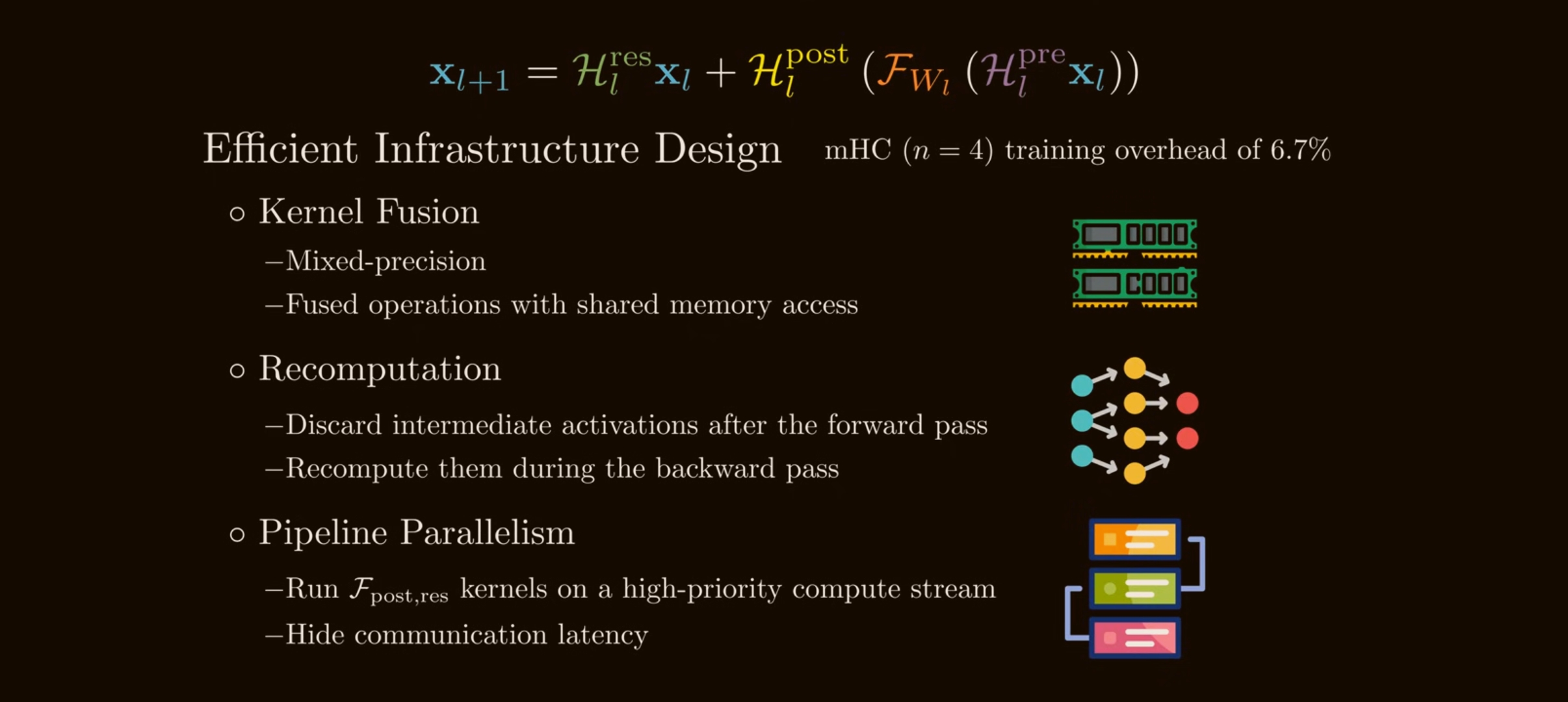
mHC’s efficiency optimizations
DeepSeek’s mHC paper adds infrastructure work to make the math practical.
Kernel fusion
mHC fuses coefficient generation, RMSNorm-related operations, Sinkhorn-Knopp, and residual merge paths where possible. In particular, it fuses the post/residual application:
\[\mathcal{F}_{\mathrm{post,res}} \mathrel{:=} \mathcal{H}_{l}^{\mathrm{res}}\mathbf{x}_l + \mathcal{H}_{l}^{\mathrm{post}\,\top}\mathcal{F}(\cdot,\cdot).\]The paper reports this reduces reads for that kernel from:
\[(3n+1)C \quad\text{to}\quad (n+1)C,\]and writes from:
\[3nC \quad\text{to}\quad nC.\]Recomputing instead of storing
Because the mHC coefficient kernels are cheaper than the attention/MLP block, the paper discards many intermediate mHC activations after the forward pass and recomputes them during backward.
For a recomputation block of $L_r$ consecutive layers, the memory objective is:
\[L_r^* = \arg\min_{L_r} \left[ nC\left\lceil\frac{L}{L_r}\right\rceil + (n+2)CL_r \right] \approx \sqrt{\frac{nL}{n+2}}.\]The first term is persistent storage for block starts. The second term is transient memory during recomputation.
The recomputation strategy is:
def backward_with_mhc_recompute(block_start_x, saved_layer_outputs, layers):
    """
    Store only block_start_x plus heavy layer outputs.
    Recreate cheap mHC maps and intermediate residual states during backward.
    """
    x = block_start_x
    states = [x]

    for layer in layers:
        h_pre, h_post, h_res = mhc_maps(x, *layer.mhc_params)
        x = h_res @ x + h_post[:, None] * saved_layer_outputs[layer.id][None, :]
        states.append(x)

    # Backprop now uses recomputed states instead of storing all of them.
    return run_backward_from_recomputed_states(states, layers)
Pipeline overlap
For large-scale distributed training, the $n$-stream state increases pipeline communication. DeepSeek extends its DualPipe schedule so mHC communication and recomputation can overlap with useful compute, especially around pipeline-stage boundaries.
The result reported for $n=4$ is only 6.7% additional training time overhead, after these optimizations.
Empirical picture
The original HC paper reports large gains in OLMo/OLMoE-style pretraining. In the OLMoE-1B-7B setting, DHC with $n=4$ converged about 1.8x faster than the baseline and improved several downstream metrics.
The mHC paper’s 27B results preserve most of the HC benefit while stabilizing training. The reported benchmark table is:
| Model | BBH | DROP | GSM8K | HellaSwag | MATH | MMLU | PIQA | TriviaQA |
|---|---|---|---|---|---|---|---|---|
| 27B Baseline | 43.8 | 47.0 | 46.7 | 73.7 | 22.0 | 59.0 | 78.5 | 54.3 |
| 27B w/ HC | 48.9 | 51.6 | 53.2 | 74.3 | 26.4 | 63.0 | 79.9 | 56.3 |
| 27B w/ mHC | 51.0 | 53.9 | 53.8 | 74.7 | 26.0 | 63.4 | 80.5 | 57.6 |
The stability story is more important than the raw score table:
- vanilla HC can outperform early, but the gradient norm and loss can surge at scale;
- mHC keeps the multi-stream expressivity while making the residual product behave like conservative mixing;
- the composite gain drops from nearly $3000$ in HC to a bounded value around $1.6$ in mHC’s finite-iteration implementation.
Why the constraint works
The key mechanism in mHC is the doubly stochastic constraint on $\mathcal{H}^{\mathrm{res}}$. Its effect is easiest to see through the residual product across depth:
- The instability is not mainly about the immediate single-layer output. It is about the product of residual mixing matrices across many layers.
- Row sums and column sums have different interpretations: row sums correspond to forward signal gain; column sums correspond to backward gradient gain.
- Doubly stochastic matrices are stable because of three linked facts: non-negativity, row/column conservation, and closure under multiplication.
- The constraint needs systems support. Without kernel fusion, recomputation, and pipeline overlap, the widened residual stream would be too I/O-heavy.
- Sinkhorn-Knopp is approximate at finite iteration count. Later variants such as mHC-lite and KromHC target exact or cheaper parameterizations of doubly stochastic residual maps.
Open engineering questions
mHC stabilizes the residual product, but it leaves several practical trade-offs.
Finite Sinkhorn iterations
With finite $t_{\max}$, Sinkhorn-Knopp only approximately reaches the Birkhoff polytope. The mHC paper uses $t_{\max}=20$, which is effective empirically, but still leaves a small approximation gap.
The mHC-lite paper proposes constructing doubly stochastic matrices directly as convex combinations of permutation matrices. This uses the Birkhoff-von Neumann theorem and avoids iterative Sinkhorn projection, but it introduces its own parameterization and engineering trade-offs.
Parameter cost of residual maps
In mHC, the residual projection uses:
\[\phi_l^{\mathrm{res}} \in \mathbb{R}^{nC\times n^2},\]so the residual-map parameterization scales like:
\[O(n^3C).\]This is manageable for small $n$, but KromHC explores Kronecker-product residual matrices to reduce complexity while preserving exact double stochasticity.
Expressivity versus constraints
Doubly stochastic matrices forbid negative mixing. This supports conservative signal propagation, but may restrict expressivity. Later work explores alternative manifolds with different stability constraints. The design pressure is the same: make the residual stream learnable without allowing depthwise composition to create pathological gain.
Summary
Hyper-Connections generalize residual connections by turning the single residual stream into $n$ streams and learning how to aggregate, update, and mix them:
\[\mathbf{x}_{l+1} = \mathcal{H}_{l}^{\mathrm{res}}\mathbf{x}_l + \mathcal{H}_{l}^{\mathrm{post}\,\top} \mathcal{F} \left( \mathcal{H}_{l}^{\mathrm{pre}}\mathbf{x}_l, \mathcal{W}_l \right).\]This gives the model a richer topology across depth. But the same flexibility creates instability because:
\[\prod_l \mathcal{H}_l^{\mathrm{res}}\]can amplify or attenuate signals exponentially.
mHC solves this by forcing:
\[\mathcal{H}_l^{\mathrm{res}} \in \left\{ H\ge 0 \mid H\mathbf{1}=\mathbf{1}, \mathbf{1}^{\top}H=\mathbf{1}^{\top} \right\}.\]The result is a residual mixer that can exchange information across streams, but whose products remain conservative and stable. The real contribution is the combination of topology, math, and systems work: widen the residual stream, constrain the dangerous map, then make the implementation bandwidth-aware.
Sources
- Defa Zhu et al., Hyper-Connections, arXiv:2409.19606.
- Zhenda Xie et al., mHC: Manifold-Constrained Hyper-Connections, arXiv:2512.24880.
- How mHC Reinvents Residual Connections, source video for the figures used in this explainer.
- Yongyi Yang and Jianyang Gao, mHC-lite: You Don’t Need 20 Sinkhorn-Knopp Iterations, arXiv:2601.05732.
- Wuyang Zhou et al., KromHC: Manifold-Constrained Hyper-Connections with Kronecker-Product Residual Matrices, arXiv:2601.21579.