Decompose-K: From torch.compile to Hand-Tuned Triton Kernels for Skinny Large‑K Matmuls
The source code for this post is available on GitHub: shreyansh26/MLSys-Experiments/decompose-k.
The idea of Decompose-K and the custom-op autotuning workflow comes from the PyTorch Conference talk Lightning Talk: Faster Than SOTA Kernels in Torch.compile With Subgraph Fusions and Custom Op Autotuning - Elias Ellison & Paul Zhang, Meta. This post is my own implementation walkthrough and benchmark study built around that idea.
The skinny large-K matmul problem
A standard matmul is
C[M, N] = A[M, K] @ B[K, N]
and the way a GPU GEMM extracts parallelism is by tiling the M x N output. Each program owns a BLOCK_M x BLOCK_N tile of C and streams over K to accumulate it. That works well when M and N are large, because there are many output tiles and the GPU has plenty of independent work to fill its streaming multiprocessors (SMs).
The problem case is a skinny, K-dominant matmul: M and N are tiny while K is huge. Think M = N = 16 with K = 32768, or a decode-time MoE router GEMM like [T, 7168] @ [7168, 256] where T can be as small as 1. Now the output is 16 x 16 = 256 elements, which is one or two tiles. The GPU has 132 SMs sitting idle while one or two programs serially walk a reduction of length 32768. The matmul is reduction-bound, but the standard tiling exposes almost no parallelism along the only large axis.
Decompose-K is a restructuring that fixes exactly this mismatch. The basic idea is simple: if the only big dimension is K, then split K and parallelize over the split.
What Decompose-K does
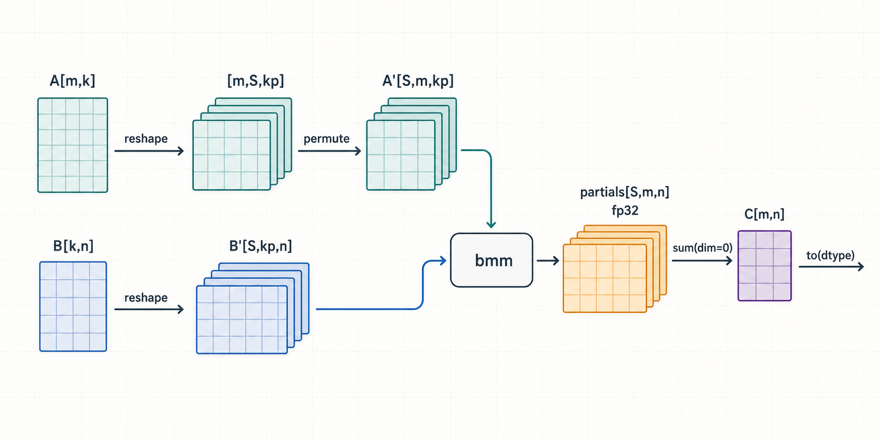
Split the K dimension into S independent chunks, compute S partial GEMMs, then sum the partials:
A[M, K] @ B[K, N]
  -> partials[S, M, N]
  -> sum(partials, dim=0)
Each partial is a smaller matmul over K/S of the reduction. The S partials are independent, so they become a batched matmul (bmm) with batch dimension S. The minimal PyTorch version makes this concrete:
def decomposeK(a, b, k_splits):
    m, k = a.shape
    n = b.shape[1]
    assert k % k_splits == 0, "k must be divisible by k_splits"
    k_parts = k // k_splits

    # [m, k] -> [m, k_splits, k_parts] -> [k_splits, m, k_parts]
    a_reshaped = a.reshape(m, k_splits, k_parts).permute(1, 0, 2)
    b_reshaped = b.reshape(k_splits, k_parts, n)        # [k_splits, k_parts, n]

    result = torch.bmm(a_reshaped, b_reshaped, out_dtype=torch.float32)
    reduced_result = result.sum(dim=0)
    return reduced_result.to(a.dtype)
The important part is what the reshape buys. For M = N = 16, K = 32768, S = 64:
-
a_reshapedis[64, 16, 512],b_reshapedis[64, 512, 16]. - The
bmmnow has 64 independent matmuls instead of one. That is 64 units of work the scheduler can spread across SMs, versus a single output tile before. - Each partial accumulates only
512of the reduction, not32768.
We have traded one long serial reduction for S short parallel ones, plus a final reduction of the S partials. The partials are accumulated in fp32 (out_dtype=torch.float32) so the split does not cost accuracy relative to a single fp32-accumulated matmul.
This is essentially split-K, but expressed at the tensor level as a bmm plus a reduction rather than as atomic adds into a single output tile. That distinction matters once we add an epilogue, which is the next point.
Why it is epilogue-friendly
A split-K design that uses atomic adds into the output has a problem if you want to fuse an elementwise epilogue like ReLU: the output tile is not final until every split has finished its atomic contribution, so you cannot apply ReLU during the accumulation. You would need a separate pass after all atomics settle.
Decompose-K keeps the partials in a separate [S, M, N] buffer and does an explicit reduction. That means the reduction step is the natural and only place where each output element becomes final, so an epilogue can be folded directly into the reduction’s store:
acc = sum over splits of partials[:, m, n]
acc = relu(acc)          # fused into the same kernel
store C[m, n] = acc
No extra pointwise pass over C, no second read/write of the output. For tiny outputs that are memory-bound on the epilogue, this is a real saving, and we will measure it later (~1.2x–1.4x over an unfused ReLU).
Where it is worth it
Decompose-K is attractive when:
-
Kis very large andM/Nare small (e.g.M = N = 16..64,K = 8192..32768). - The workload is latency-sensitive and a single fixed shape matters more than a general GEMM. A concrete example is a DeepSeek-V3 MoE router GEMM
[T, 7168] @ [7168, 256], where decode has tiny dynamicT = 1..256and prefill has largerT. - A fused epilogue like ReLU can ride along on the reduction.
It is not worth it when M and N are already large enough to fill the GPU, when K is small, when K divides poorly for the candidate split counts, or when the extra [S, M, N] buffer and its reduction dominate the cost.
The rest of this post is a tour of implementations of this one idea, from the laziest (torch.compile) to a hand-written Triton kernel that beats Inductor’s own autotuned choice. Every benchmark below is BF16 on an H100 (132 SMs), over the grid M = N ∈ {16, 32, 48, 64} and K ∈ {8192, …, 32768}.
Baseline: just call torch.compile
The first thing to try is to write decomposeK in plain PyTorch and let Inductor handle the rest. The relevant detail is the compile mode. Across the three benchmark suites used throughout this post - a BF16 matmul with a fused ReLU epilogue (epilogue-bf16), a plain BF16 matmul (matmul-bf16), and a plain FP32 matmul - max-autotune-no-cudagraphs was the best mode, edging out max-autotune:
decomposeK_compiled = torch.compile(decomposeK, mode="max-autotune-no-cudagraphs")
max-autotune turns on Inductor’s template autotuning (it benchmarks several generated kernels and picks the fastest). The -no-cudagraphs variant skips CUDA graph capture, which for these tiny single-shot calls avoids capture overhead without losing the autotuning benefit.
What does naive compilation actually emit?
Compiling the decomposeK function above (for the router shape [64, 7168] @ [7168, 256], S = 4) produces two operations, which you can read off the Inductor output code:
# extern bmm into an fp32 partials buffer
buf0 = empty_strided_cuda((4, 64, 256), (16384, 256, 1), torch.float32)
extern_kernels.bmm_dtype(
    reinterpret_tensor(arg0_1, (4, 64, 1792), ...),
    reinterpret_tensor(arg1_1, (4, 1792, 256), ...),
    out_dtype=torch.float32, out=buf0)

# one generated pointwise kernel: sum over the 4 splits + cast to bf16
triton_poi_fused__to_copy_sum_0.run(buf0, buf1, 16384, ...)
So the bmm goes to an external (cuBLAS) batched kernel, and the sum(dim=0) plus the .to(bf16) cast get fused into a single generated Triton pointwise kernel. The generated reduction kernel is literally an unrolled add of the S = 4 slices:
tmp0 = tl.load(in_ptr0 + (x0), None)
tmp1 = tl.load(in_ptr0 + (16384 + x0), None)
tmp3 = tl.load(in_ptr0 + (32768 + x0), None)
tmp5 = tl.load(in_ptr0 + (49152 + x0), None)
tmp7 = (tmp0 + tmp1 + tmp3 + tmp5)
tl.store(out_ptr0 + (x0), tmp7, None)
This is the call graph for explicit Decompose-K written in PyTorch: bmm + a fused sum/cast kernel. If instead you write the version with a ReLU epilogue, the fused kernel additionally folds in maximum(0, x), so you get bmm + a fused sum+relu kernel. The epilogue is free in the sense that it rides on the reduction kernel that has to run anyway.
What if you just write relu(mm(a, b)) and let Inductor decide?
This is the more interesting question, because the PyTorch nightly used here (torch==2.12.0.dev20260408+cu128) ships a Decompose-K lowering inside Inductor itself - see torch/_inductor/template_heuristics/decompose_k.py and the subgraph choice it registers in torch/_inductor/kernel/mm.py. So Inductor will reach for the decomposition on large-K shapes on its own, autotuning it as one more candidate against the regular matmul templates. The POC compiles a plain torch.relu(torch.mm(a, b)) and dumps the generated code at two K values.
Small K (M = N = 16, K = 256) - Inductor emits a single fused matmul template, triton_tem_fused_mm_relu_0, with the source nodes [aten.mm, aten.relu]. The ReLU is fused into the matmul template’s store suffix:
# inductor's template suffix, inside the matmul kernel
tmp1 = triton_helpers.maximum(tmp0, acc)   # relu
tl.store(out_ptr1 + xindex, tmp1, mask)
One kernel, ReLU fused, done. There is no reason to decompose at small K.
Large K (M = N = 16, K = 32768) - Now Inductor chooses Decompose-K on its own. The generated graph is named decompose_k_mm_64_split_5 (it picked S = 64, so k_part = 512) and contains three pieces:
# 1) batched partial matmul via cuBLAS, fp32 accumulate
extern_kernels.bmm_dtype(
    reinterpret_tensor(arg0_1, (64, 16, 512), ...),
    reinterpret_tensor(arg1_1, (64, 512, 16), ...),
    out_dtype=torch.float32, out=buf0)         # buf0: [64, 16, 16] fp32

# 2) generated reduction over the 64 splits
triton_per_fused_mm_0.run(buf0, buf2, 256, 64, ...)

# 3) a SEPARATE pointwise relu kernel
triton_poi_fused_relu_1.run(buf1, 256, ...)
The thing to notice is piece 3. When Inductor takes the Decompose-K lowering, it emits ReLU as a separate triton_poi_fused_relu_1 pointwise kernel after the reduction. It does not fuse ReLU into the Decompose-K reduction/store. That is an extra full read-and-write of the output buffer. For a tiny 16 x 16 output this is small in absolute terms, but it is exactly the fusion opportunity a hand-written kernel can reclaim, and it is the gap the rest of this post chases.
So we have two facts to build on: Decompose-K is the right structure at large K (Inductor agrees), and the stock Inductor lowering leaves the epilogue unfused. Time to write the kernel ourselves.
A hand-written Triton kernel
Source: kernels/decompose_k_triton_kernel.py
The kernel is two stages that mirror the structure above: a partial-matmul kernel that fills [S, M, N], and a reduction/epilogue kernel that sums over S and optionally applies ReLU on the store.
Stage 1: partial matmul
The partial-matmul kernel uses a 2D launch grid: program_id(0) indexes the M x N output tile (with the usual L2-friendly group-major swizzle), and program_id(1) indexes the split. Each program computes one BLOCK_M x BLOCK_N tile for one split, accumulating only its K // SPLIT_K slice of the reduction.
@triton.jit
def _partial_mm(a, b, partials, ...):
    pid = tl.program_id(0)
    split_id = tl.program_id(1)

    # group-major swizzle of pid -> (pid_m, pid_n) for L2 reuse
    ...
    offs_m = pid_m * BLOCK_M + tl.arange(0, BLOCK_M)
    offs_n = pid_n * BLOCK_N + tl.arange(0, BLOCK_N)
    offs_k = tl.arange(0, BLOCK_K)

    k_per_split = K // SPLIT_K
    split_k_start = split_id * k_per_split
    acc = tl.zeros((BLOCK_M, BLOCK_N), tl.float32)

    for k0 in range(0, k_per_split, BLOCK_K):
        k_offsets = k0 + offs_k
        a_ptrs = a + offs_m[:, None] * stride_am + (split_k_start + k_offsets[None, :]) * stride_ak
        b_ptrs = b + (split_k_start + k_offsets[:, None]) * stride_bk + offs_n[None, :] * stride_bn
        k_mask = k_offsets < k_per_split
        a_vals = tl.load(a_ptrs, mask=(offs_m[:, None] < M) & k_mask[None, :], other=0.0)
        b_vals = tl.load(b_ptrs, mask=k_mask[:, None] & (offs_n[None, :] < N), other=0.0)
        acc += tl.dot(a_vals, b_vals, out_dtype=tl.float32, input_precision=INPUT_PRECISION)

    partial_ptrs = partials + split_id * stride_ps + offs_m[:, None] * stride_pm + offs_n[None, :] * stride_pn
    tl.store(partial_ptrs, acc, mask=(offs_m[:, None] < M) & (offs_n[None, :] < N))
A few details worth calling out:
- The accumulator is fp32 regardless of input dtype, and
input_precisionis"ieee"for fp32 inputs and"tf32"otherwise. This keeps the split from changing numerical behaviour versus a single accumulated matmul. -
split_k_start = split_id * k_per_splitis the only thing that distinguishes one split program from another. Each split reads a contiguousk_per_splitband ofK. - The store writes into the split-indexed
partials[split_id]slice. There are no atomics: every(split_id, tile)pair owns a disjoint region of the partials buffer.
Stage 2: reduce + fused epilogue
The reducer launches one program per output tile, loops over all SPLIT_K partials into a tile-shaped accumulator, applies ReLU if requested, and stores:
@triton.jit
def _reduce_epilogue(partials, c, ..., SPLIT_K, BLOCK_M, BLOCK_N, FUSE_RELU):
    # (pid -> pid_m, pid_n) swizzle as before
    ...
    acc = tl.zeros((BLOCK_M, BLOCK_N), tl.float32)
    for split_id in range(0, SPLIT_K):
        acc += tl.load(ptrs + split_id * stride_ps,
                       mask=(offs_m[:, None] < M) & (offs_n[None, :] < N), other=0.0)

    if FUSE_RELU:
        acc = tl.maximum(acc, 0.0)

    tl.store(c_ptrs, acc, mask=(offs_m[:, None] < M) & (offs_n[None, :] < N))
This is the fusion that Inductor’s Decompose-K lowering does not do: ReLU is applied in registers before the single store of C, with no separate pointwise pass. Correctness-wise, this is safe precisely because the explicit reduction is where each output element first becomes final.
This kernel is correct and reasonable, but it carries a structural limitation in how the reducer is parallelized - one we will pin down in a moment. Because the surprising part comes first: this hand-written kernel does not actually beat Inductor.
Custom-op autotuning: letting Inductor pick the decomposition
Source: custom_op_autotune_relu_dispatch.py
Inductor exposes an API, register_custom_op_autotuning, that lets you hand it a list of alternative decompositions for an op and have it benchmark and select among them per shape, then lower the winner. The neat trick is that the target op can be either a real @torch.library.custom_op or an existing ATen overload like torch.ops.aten.mm.default. So you can intercept the lowering of every torch.mm in a compiled graph.
The candidates are plain mm (or mm + relu) plus one Decompose-K decomposition per valid split count:
K_SPLITS = (2, 4, 8, 16, 32, 64, 128, 256)

def generate_mm_relu_configs(fake_tensors):
    k = int(fake_tensors["a"].shape[1])
    splits = [s for s in K_SPLITS if k % s == 0]
    configs = [CustomOpConfig(mm_relu_impl)]
    configs += [CustomOpConfig(decompose_k_relu_impl, k_splits=s) for s in splits]
    return configs
decompose_k_relu_impl is just the PyTorch-level bmm + sum + relu from the start of the post; we are not handing Inductor a Triton kernel here. We are handing it several mathematically-equivalent PyTorch decompositions and letting it lower and time each one.
The script registers this at two different boundaries, each with a matching config generator, so both the plain-matmul and the fused matmul+ReLU cases are covered:
-
aten.mmboundary -generate_mm_configs, keyedself/mat2. Candidates aremm_impl(the ordinarytorch.mmlowering) plusdecompose_k_impl(k_splits=s)for everysinK_SPLITSthat dividesK. ReLU stays outside the autotuned op as a separate pointwise kernel. - fused
mm_relucustom-op boundary -generate_mm_relu_configs, keyeda/b. Candidates aremm_relu_impl(plainrelu(mm)) plusdecompose_k_relu_impl(k_splits=s)for each valids- the ReLU is folded into every candidate, so Inductor times the fully fused decomposition directly.
The shape of the candidate list is the same either way: the plain lowering plus one Decompose-K candidate per valid split count. Decompose-K is never special-cased - it is just one more entry in the menu that has to win the autotune on its own merits at each shape.
The registration wires up the autotuning:
register_custom_op_autotuning(
    custom_op=torch.ops.aten.mm.default,    # intercept every torch.mm
    config_generator=generate_mm_configs,   # candidates from fake-tensor shapes
    name="router_mm_relu_autotune",
    input_gen_fns={                          # make real CUDA tensors to benchmark
        "self": lambda fake: torch.randn_like(fake, device="cuda") * 0.1,
        "mat2": lambda fake: torch.randn_like(fake, device="cuda") * 0.1,
    },
    dispatch_on={"tensor_name": "self", "dim": 0, "range_upper_bound": 1024},
    split_points=[1, 8, 32, 128, 512],
    benchmark_with_cudagraphs=True,
)
The pieces that matter:
-
config_generatorreceives fake tensors keyed by the op’s schema argument names (self/mat2foraten.mm) and returns candidates for the current compile shape. This is how it inspectsKand only emits splits whereK % k_splits == 0. -
input_gen_fnsturn the fake tensors into real CUDA tensors so each candidate can actually be timed. The keys must match the ATen schema names. -
dispatch_on+split_pointsenable range-based dispatch. Here it benchmarks and dispatches onself.shape[0], i.e. theM/Tdimension.split_points = [1, 8, 32, 128, 512]becomes ranges roughly[1,1], [2,8], [9,32], [33,128], [129,512], [513, inf]. Inductor picks a winner per range and, if adjacent ranges want different winners, emits a runtimetorch.conddispatch tree. This is the “custom op dispatching per dynamic shape” idea: decode (T=1) and prefill (Tlarge) can get different kernels from the same compiled graph.
So there are two layers of timing in the benchmark. First, Inductor autotunes during compile and lowers a winner. The harness captures that decision into the CSV: across the whole grid, the winner was decompose_k_relu_impl with k_splits of 64 or 128 (it agrees that Decompose-K is right). Second, the harness times the already-compiled callable with do_bench.
Two ways to use the registration: one graph for all shapes, or one per shape
The registration is used in two different ways.
Standalone, custom_op_autotune_relu_dispatch.py runs the dynamic path: it registers with dispatch_on + split_points, compiles with dynamic=True, and sweeps T = [1, 16, 64, 256, 768] against eager. Here the torch.cond per-M dispatch tree matters - one compiled graph routes decode-like (T = 1) and prefill-like (T large) shapes to whatever candidate won their range.
The benchmark measures one fixed shape at a time, so it skips that path. bench_decompose_k.py resets Dynamo (torch._dynamo.reset()) before each grid point and compiles with dynamic=False, so Inductor specializes for the exact (M, K, N). It registers the static variants (register_mm_relu_static_autotune / register_mm_static_autotune), which leave out dispatch_on and split_points: with a single shape there is no range to cover and no torch.cond tree, so each shape is autotuned and lowered on its own and the harness records the winner. Range-based dispatch belongs to the standalone exploration; it plays no part in the Results numbers below.
An easy way to mis-benchmark: the Dynamo recompile limit
This grid is easy to mis-benchmark. torch.compile specializes the same Python function over many exact shapes, and TorchDynamo’s default config.recompile_limit is 8 per code object. If you keep recompiling for new K without resetting Dynamo, you eventually hit:
torch._dynamo hit config.recompile_limit (8)
After that, later shapes stop getting fresh optimized graphs and silently fall back to slower execution, which makes the recorded custom-op timing (the custom_op_mm_relu_ms column in the benchmark CSV) look great for the first few shapes and then jump up to the eager band. That is a benchmark cache artifact, not the candidate getting slower. The fix is to reset Dynamo between exact-shape grid points before compiling the next measured callable (compile time is not part of the latency measurement, so this is fair).
Limitations of the hand-written kernel
How does our hand-written baseline Triton kernel compare against this custom-op autotuned path? It loses, everywhere:
| Suite | Wins (standalone vs custom-op) | min / median / max speedup |
|---|---|---|
epilogue-bf16 | 0 / 28 | 0.874x / 0.917x / 0.982x |
matmul-bf16 | 0 / 28 | 0.886x / 0.920x / 0.956x |
Speedup is custom_op_mm_relu_ms / decompose_k_fused_ms, using the column names in the benchmark CSV - the standalone kernel is logged as decompose_k_fused_ms or decompose_k_unfused_ms depending on whether ReLU is fused into the reduction, and as decompose_k_ms in the plain matmul-bf16 suite. Below 1.0x means the standalone kernel is slower. Inductor’s lowering of the same Decompose-K math beats our kernel by ~8–13% on the median. The reason is the reducer - the structural limitation hinted at earlier.
Our reducer is output-tile shaped: one program owns a BLOCK_M x BLOCK_N tile, carries a 2D accumulator of that shape, and serially walks the split dimension in a Python-level for loop. For a tiny output like M = N = 16, a 16 x 16 reducer tile can mean a single reducer program for the whole output, and that one program serially reads all SPLIT_K partials. The reduction parallelism is tied to the matmul output tiling, which is the wrong axis to parallelize when the output is tiny and the split count is large.
Inductor sidesteps exactly this: its generated reduction (a triton_per_fused persistent reduction over the split axis) parallelizes the split correctly. The matmul template is roughly a wash; the reduction is where we are losing - and that is precisely what the optimized kernel fixes next.
The optimized Triton kernel
Source: kernels/decompose_k_triton_kernel_optimized.py
The optimized kernel keeps the same two-stage structure (and reuses the exact same _partial_mm) but rewrites the reducer and widens the autotuning search. There are four changes.
1. Reshape the reducer around the split axis
This is the big one. Instead of an output-tile-shaped accumulator that serially loops over splits, flatten the output matrix into a 1D element index x = m * N + n and treat the split as the reduction axis of a proper 2D vector reduction:
vals: [XBLOCK, RBLOCK]   # XBLOCK output elements x RBLOCK splits
acc:  [XBLOCK]           # one fp32 result per output element
Each reducer program owns a disjoint slice of XBLOCK flattened output elements, loads all RBLOCK (= SPLIT_K, padded to a power of two) partials for them, and reduces with a single tl.sum over the split axis:
@triton.jit
def _reduce_epilogue_vector_flat(partials, c, stride_ps, XNUMEL, SPLIT_K, XBLOCK, RBLOCK, FUSE_RELU):
    x_base = tl.program_id(0) * XBLOCK + tl.arange(0, XBLOCK)
    x = x_base[:, None]
    r = tl.arange(0, RBLOCK)[None, :]
    vals = tl.load(partials + r * stride_ps + x,
                   mask=(x < XNUMEL) & (r < SPLIT_K), other=0.0)
    acc = tl.sum(vals, 1)                  # vector reduction over splits
    if FUSE_RELU:
        acc = tl.maximum(acc, 0.0)
    tl.store(c + x_base, acc, mask=x_base < XNUMEL)
For M = N = 16 (256 output elements) with XBLOCK = 32, this launches 8 reducer programs, each owning 32 elements and reducing all splits for them in one vectorized sum. There is no cross-program combine step: every program writes final values directly. Crucially, this decouples reducer tiling from matmul tiling: the partial matmul can use 16x16 or 64x64 tiles while the reducer independently uses a small XBLOCK chosen for split-reduction efficiency.
2. A flat contiguous fast path
For the common case of contiguous row-major tensors, the address math collapses. Because partials[s, m, n] lives at base + s*(M*N) + (m*N + n) and x = m*N + n, the hot loads and stores are just partials + r * stride_ps + x and c + x_base - no division/modulo to recover (m, n):
if partials.is_contiguous() and c.is_contiguous():
    _reduce_epilogue_vector_flat[grid](...)   # no (m,n) reconstruction
else:
    _reduce_epilogue_vector[grid](...)        # general strided fallback
The strided kernel (with the x // N, x - m*N reconstruction) stays as a fallback for non-contiguous views like c = base[:, ::2].
3. Warp counts matched to tiny tiles
The baseline search used 4 warps everywhere. But a 16x16 output tile has only 256 fp32 accumulators; even with a K slice of 64–128, a partial-matmul program for that tile is too small to keep 4 warps (128 threads) busy. Four warps there means more scheduling/sync overhead, more register pressure, and fewer resident programs per SM - the opposite of what a tiny-output, large-K shape calls for.
So the optimized config set deliberately includes 1- and 2-warp small tiles (16x16x64, 16x16x128, …) alongside 4-warp larger tiles (64x32, 64x64, …). The intuition is work per program:
16x16x128 =  32,768 multiply-add positions   -> few warps
64x32x64  = 131,072 multiply-add positions
64x64x128 = 524,288 multiply-add positions   -> 4 warps pay off
Both families are in the search, and the benchmark picks per shape. (In the results, small M=N tend to pick 16x16 tiles, while M=N=64 shifts to 64x32/64x64.)
4. More split candidates
The optimized split search explicitly tries the power-of-two counts (2, 4, 8, 16, 32, 64, 128, 256) and then appends the baseline divisor-based candidates. This matches the custom-op setup and maps naturally onto the power-of-two RBLOCK the vectorized reducer uses for the split axis.
Now it wins
With the vectorized reducer, the standalone kernel flips from losing everywhere to winning almost everywhere against the custom-op autotuned path:
| Suite | Wins (standalone vs custom-op) | min / median / max speedup |
|---|---|---|
epilogue-bf16 | 26 / 28 (+1 tie) | 0.990x / 1.026x / 1.080x |
matmul-bf16 | 24 / 28 (+2 ties) | 0.997x / 1.022x / 1.052x |
The reducer rewrite alone moved the median from 0.917x to 1.026x on the epilogue suite - roughly an 11% swing, recovered entirely from how the split reduction is parallelized and from folding ReLU into the store instead of running Inductor’s separate pointwise pass.
Benchmark setup
A few details about how the numbers below are produced, since they affect what the comparison actually measures.
One fresh compile per shape - The grid sweeps M = N ∈ {16, 32, 48, 64} against K ∈ {8192, 12288, 16384, 20480, 24576, 28672, 32768} - 28 shapes per suite. For every shape the harness calls torch._dynamo.reset() and then torch.compile(target, mode="max-autotune-no-cudagraphs", dynamic=False). The reset clears the compile cache so the recompile limit from earlier never triggers, and dynamic=False lets Inductor specialize fully for that one (M, N, K) instead of generating a shape-generic kernel. The cost is one autotuning pass per shape, but the payoff is that each point in the grid reflects the best kernel Inductor can produce for exactly that shape - which is the fairest thing to compare a hand-tuned kernel against. For FP32 runs the harness also sets torch.set_float32_matmul_precision("highest") (and "high" otherwise) so the matmul precision matches the chosen dtype.
Timing - Latency comes from triton.testing.do_bench(fn, warmup=10, rep=50, return_mode="median") - 10 warmup iterations, 50 measured, reported as the median. do_bench handles the L2-cache flush and CUDA-event timing internally, so the numbers are wall-clock kernel time without host overhead. Every candidate is also checked for correctness with torch.testing.assert_close (tolerances per dtype) before it is timed, so a config that diverges numerically is rejected rather than ranked.
Data types - The post shows two suites: epilogue-bf16 (a BF16 matmul with a fused ReLU epilogue) and matmul-bf16 (plain BF16 matmul, no epilogue). The repo runs two more that are not plotted here - matmul-fp16 (plain FP16 matmul) and matmul-fp32 (plain FP32 matmul, with tighter rtol=1e-4/atol=1e-3 tolerances). The FP16 picture matches BF16 closely; FP32 has less to gain because the larger element size and tighter accumulation leave less headroom for the split reduction, but the ordering is the same.
Results
All raw numbers and plots are checked into the repo, so the runs are reproducible and inspectable: the original hand-written kernel lives under bench_results/ and the optimized kernel under bench_results_v2/. Each suite has a .csv with per-shape timings (eager_ms, compiled_ms, custom_op_mm_relu_ms, decompose_k_fused_ms, decompose_k_unfused_ms, …) and the captured autotune winner, plus per-M=N and overall-grid plots.
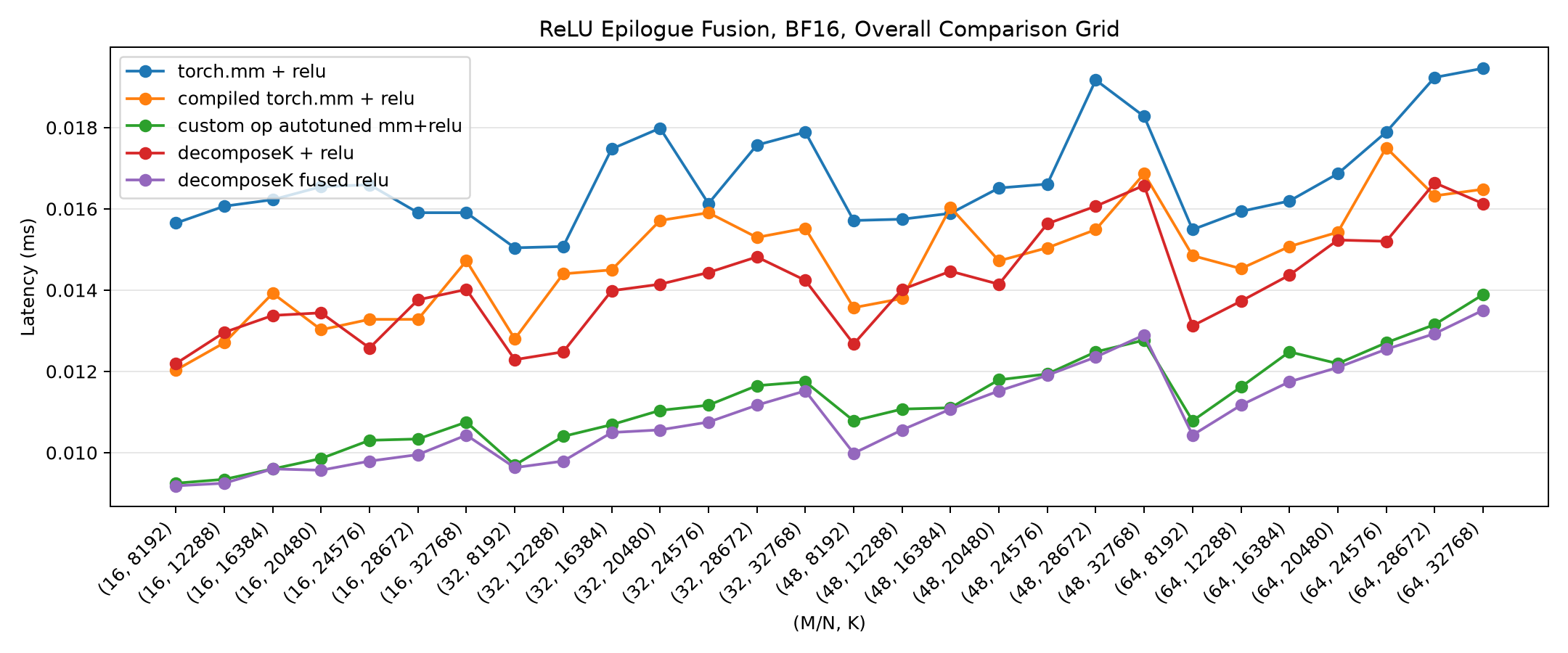
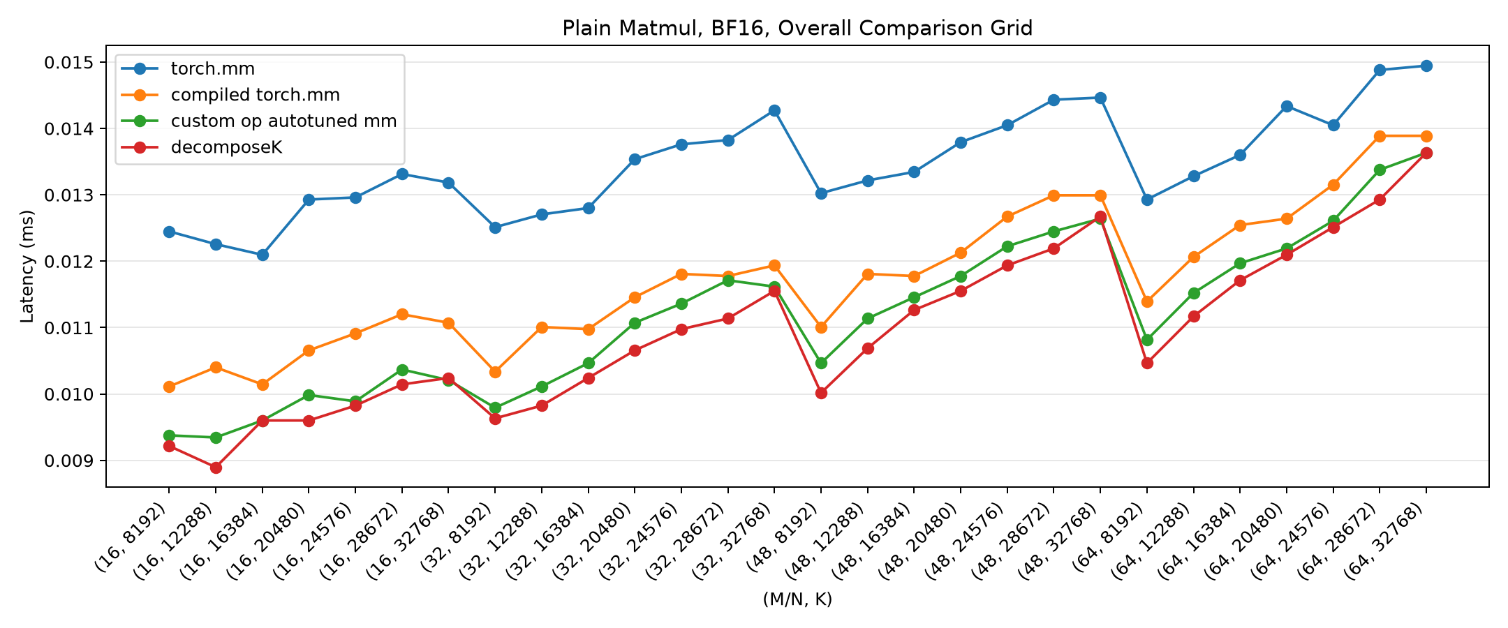
The clearest way to see the whole picture is the overall comparison grid. Each x-axis point is a (M=N, K) shape; lower latency is better. Five curves: eager torch.mm + relu, compiled torch.mm + relu, the custom-op autotuned mm+relu, standalone Decompose-K with a separate ReLU, and standalone Decompose-K with fused ReLU.
First, the original standalone Triton kernel (red/purple sit in the middle of the pack, above the green custom-op line - the kernel is not yet competitive):
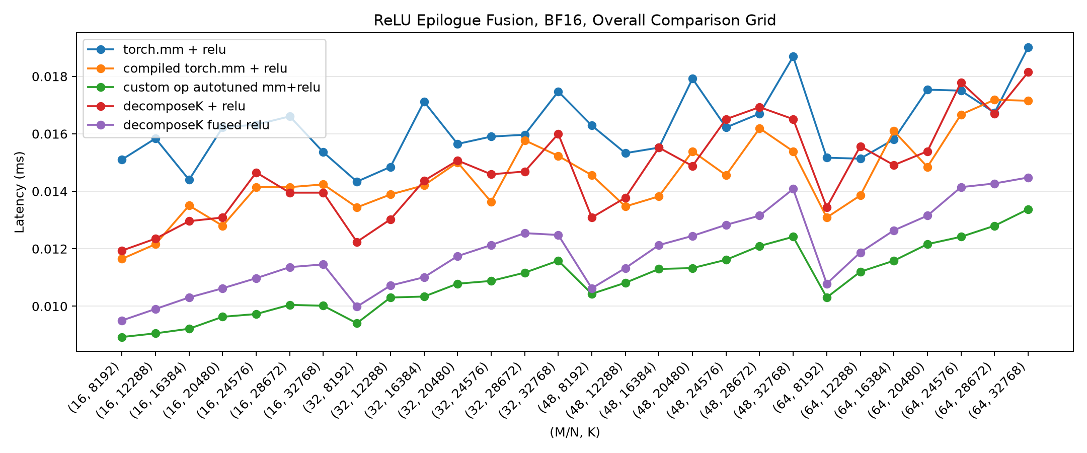
Then the optimized kernel. The fused Decompose-K curve (purple) drops to the bottom of the grid, at or below the green custom-op line across nearly all shapes:
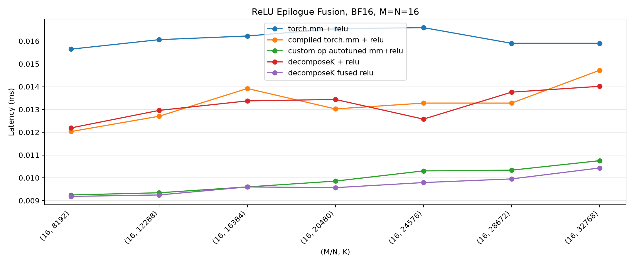
Zooming into M = N = 16, the most reduction-bound slice, makes the ordering crisp: eager (blue) is slowest, compiled and separate-ReLU Decompose-K (orange/red) are in the middle, and the fused Decompose-K (purple) and custom-op (green) share the floor - with the fused kernel slightly ahead at small K:
The plain matmul suite (no epilogue) tells the same story with a smaller margin, since there is no epilogue to fuse - the win there is purely from the reducer:
A few representative numbers from the epilogue-bf16 runs - a BF16 matmul with a fused ReLU epilogue (do_bench median, ms):
| M=N | K | eager mm+relu | compiled mm+relu | custom-op | Decompose-K fused | Decompose-K fused vs unfused |
|---|---|---|---|---|---|---|
| 16 | 8192 | 0.0156 | 0.0120 | 0.0092 | 0.0092 | 1.33x |
| 16 | 32768 | 0.0159 | 0.0147 | 0.0108 | 0.0104 | 1.34x |
| 32 | 16384 | 0.0175 | 0.0145 | 0.0107 | 0.0105 | 1.33x |
| 64 | 32768 | 0.0195 | 0.0165 | 0.0139 | 0.0135 | 1.19x |
Two things to read off this table. The fused Decompose-K kernel is consistently the fastest column, ~1.5–1.7x over eager and ~1.2–1.4x over compiled torch.mm + relu. And the last column - the fusion benefit alone, measured as the same Decompose-K config with ReLU as a separate in-place op versus fused into the reduction store - is a steady 1.19x–1.4x. That is the concrete payoff of the epilogue-friendliness from the very first section.
Takeaways
- Decompose-K is a structural fix for a structural problem. When the only large dimension is
K, splitting it turns one long serial reduction intoSparallel partial GEMMs plus a reduction, giving the GPU work to fill its SMs. It is most useful for skinny, large-K, latency-sensitive shapes (MoE routers, small-batch decode). - It is epilogue-friendly by construction. Keeping partials in a separate buffer and doing an explicit reduction means the reduction’s store is the natural place to fuse ReLU - worth ~1.2–1.4x here. A split-K-with-atomics design cannot do this cleanly.
-
torch.compilealready knows the trick. At largeK, Inductor picks Decompose-K on its own (extern bmm_dtype+ a generated reduction). But it emits the epilogue as a separate pointwise kernel, leaving the fusion on the table. - Custom-op autotuning is a strong, low-effort baseline. Handing Inductor a list of PyTorch decompositions and a per-range dispatch policy beat a naive hand-written Triton kernel on every shape. If you only do one thing, do this.
- Beating it required getting the reducer right. The win was not in the matmul; it was reshaping the reduction around the split axis (a real
tl.sumover splits, decoupled from matmul tiling), matching warp counts to tiny tiles, and folding ReLU into the store. That moved the standalone kernel from0/28to26/28wins versus Inductor’s own choice.
It is worth being honest about the effort-to-reward ratio. The hand-written kernel wins, but only by a few percent over custom-op autotuning, and getting there meant rewriting the reducer and widening the search. For most situations, staying with torch.compile is perfectly reasonable - as long as it is done carefully. Plain torch.compile(decomposeK) was not enough on its own; Inductor decomposes but leaves the epilogue as a separate kernel, and it was that gap that pushed me toward custom-op autotuning. Set up that way, the compiler does a great job, and the hand-written kernel is the last few percent you reach for only when the shape is fixed and the latency genuinely matters.
And this gap is not fundamental. The day Inductor’s Decompose-K lowering learns to fuse the epilogue into the reduction store - the same optimization the hand-written kernel relies on - most of this margin trims away on its own, and the compiler path absorbs the win for free.
All the kernels, the custom-op autotuning setup, the benchmark harness, and the raw results are on GitHub: shreyansh26/MLSys-Experiments/decompose-k.