Paper Summary #8 - FlashAttention: Fast and Memory-Efficient Exact Attention with IO-Awareness
Paper: FlashAttention: Fast and Memory-Efficient Exact Attention with IO-Awareness
Link: https://arxiv.org/abs/2205.14135
Authors: Tri Dao, Daniel Y. Fu, Stefano Ermon, Atri Rudra, Christopher Ré
Code: https://github.com/HazyResearch/flash-attention
I have also released an annotated version of the paper. You can find it here.
[Update] - I implemented a simplified version of FlashAttention (without the CUDA and SRAM memory optimizations) in PyTorch. Check it out on Github.
I finished reading the FlashAttention paper recently and thought that it would be good to have a technical write-up of the paper, so that it can help me understand the concept well. I decided to make it public and hopefully it can help anyone reading this.
Overview
Attention as we know, in its standard implementation is an \(O(N^2)\) operation, where N is the sequence length. There are many approximate attention methods out there like Reformer, SMYRF, Performer and others (you can find more details on a few of these in my previous blog) which aim to reduce the compute requirements to linear or near-linear in sequence length, but many of them do not display wall-clock speedup against standard attention. They focus on FLOP reduction (which doesn’t always correlate with wall-clock speed) and tend to ignore overheads from memory access (IO). FlashAttention aims to incorporate IO-awareness i.e. dividing operations between faster and slower levels of GPU memory to make the whole computation faster. The algorithm uses tiling to reduce the number of memory reads/writes between GPU high bandwidth memory (HBM) and GPU on-chip SRAM. FlashAttention can also be extended to block-spare attention and this results in the fastest approximate (or not) attention algorithm out there.
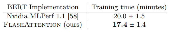
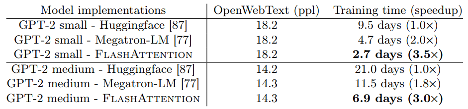
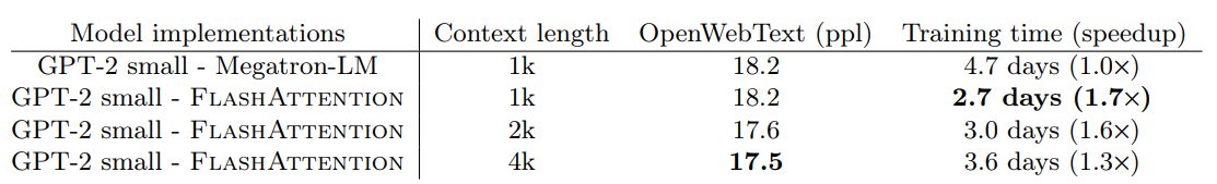
All this helps to improve the training time of Transformer models - a 15% end-to-end wall-clock speedup on BERT-large (seq. length 512) compared to the MLPerf 1.1 training speed record, 3× speedup on GPT-2 (seq. length 1K). This memory-efficient approach also helps to incorporate a longer context (up to 16k/64k tokens) which also results in better models (0.7 better perplexity on GPT-2).
I’ll describe more details in the future sections.
Background - Hardware Performance
Since FlashAttention computes exact attention, and the major crux of their work is the efficient hardware usage, it is important to know a bit about GPU memory and the performance characteristics of various kinds of operations on it.
GPU Memory Hierarchy
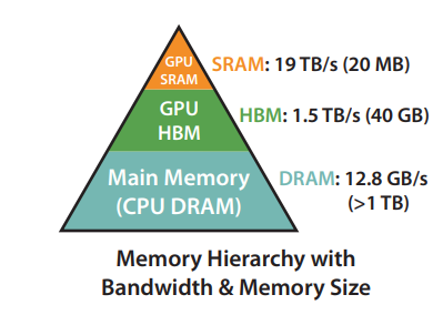
For a A100 GPU with 40GB of High Memory Bandwidth (HBM), a rough diagram of the memory hierarchy is shown above. The SRAM memory us spread across 108 streaming multiprocessors (SMs), 192KB for each. As one can see, the on-chip SRAM is much faster the HBM but is much smaller than size. In terms of compute, the theoretical peak throughput for BFloat16 using Tensor Core is 312 TFLOPS. With time, compute has gotten much faster relative to memory speed, hence processes (operations) are increasingly bottlenecked by memory (HBM) access. Thus, the goal of the FlashAttention paper was to use the SRAM as well as efficiently as possible to speed up the computation.
Execution Model
The typical way in which GPUs operate are that they use a large number of threads to perform an operation, which is called a kernel. The input is loaded from the HBM to the registers and SRAM, and written back to the HBM after computation.
Performance Characteristics
There is a term called arithmetic intensity which is given by the number of arithmetic operations per byte of memory access. It helps to understand the bottleneck of an operation. An operation can be characterized as compute-bound (also called math-bound) or memory-bound.
-
Compute-bound - When the bottleneck is the compute i.e., the time taken by the operation is determined by how many arithmetic operations there are since the time taken due to HBM accesses is relative lower. E.g. of such operations are matrix multiplication with large inner dimension, and convolution with large number of channels.
-
Memory-bound - When the bottleneck is the memory i.e., the time taken by the operation is determined by the number of memory accesses there are since the time spent in computation is relative lower. E.g. of such processes are most other operation like elementwise operations - activation, dropout and reduction operations - sum, softmax, batch normalization, layer normalization.
To understand this better, let’s analyze it mathematically. Let \(N_{op}\) be the number of arithmetic/floating point operations, \(N_{byte}\) be the number of memory accesses, \({BW}_{compute}\) and \({BW}_{memory}\) be the compute and memory bandwidth respectively, the time taken for compute operations and memory accesses can be determined as -
\[\\ \begin{align} t_{compute} = \frac{N_{op}}{BW_{compute}} \\ t_{memory} = \frac{N_{byte}}{BW_{memory}} \end{align} \\\]The operation is compute-bound if \(t_{compute}\) is greater than \(t_{memory}\) and vice-versa for memory bound. Which mathematically becomes -
For compute-bound
\(\\ \begin{align} \frac{N_{op}}{N_{byte}} \gt \frac{BW_{compute}}{BW_{memory}} \end{align} \\\)
For memory-bound
\(\\ \begin{align} \frac{N_{op}}{N_{byte}} \lt \frac{BW_{compute}}{BW_{memory}} \end{align} \\\)
As mentioned above as well, matrix multiplication for large inner dimensions is compute bound but below that it is memory bound. If using FP32 and plugging in numbers for A100 40GB, then for \(N \lt 74\), the \(N \times N\) multiplication is memory bound, but compute bound when \(N\) is greater than that. A great and detailed resource to understand this theory is this blog post by Lei Mao.
Kernel Fusion
Kernel Fusion is often down by compilers to fuse together multiple elementwise operations. It is used to accelerate memory-bound operations. The basic ideas is that instead of loading the input from the HBM, performing the operation and writing back to the HBM and repeating that for each operation applied to the same input, the operation can be fused so that all of the operations are performed at once when the input is loaded from the HBM.
However, one must note that when performing model training, the effectiveness of kernel fusion is reduced as the intermediate values still have to be written to the HBM to save for the backward pass.
Background - Standard Attention
For anyone familiar with transformers, this equation is well-known -
\[Attention(Q, K, V) = softmax(\frac{QK^\mathsf{T}}{\sqrt{d_k}})V\]Here, the sequences \(Q, K, V \in \mathbb{R}^{N \times d}\) where \(N\) is the sequence length and \(d\) is the head dimension. The attention output, above, can be denoted by \(O \in \mathbb{R}^{N \times d}\). The equation can be broken down as -
\[\mathbf{S} = \mathbf{QK^\mathsf{T}} \in \mathbb{R}^{N \times N},\quad \mathbf{P} = softmax(\mathbf{S}) \in \mathbb{R}^{N \times N},\quad \mathbf{O} = \mathbf{PV} \in \mathbb{R}^{N \times d}\]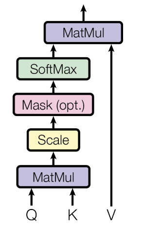
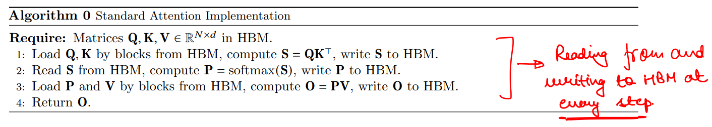
In standard attention implementations, the \(\mathbf{S}\) and \(\mathbf{P}\) matrices are materialized in the HBM, which takes \(O(N^2)\) memory. Also, most operations are memory-bound/elementwise operations, e.g. softmax applied on \(\mathbf{P}\), masking applied to \(\mathbf{S}\), dropout applied to \(\mathbf{P}\). This leads to slow wall-clock time.
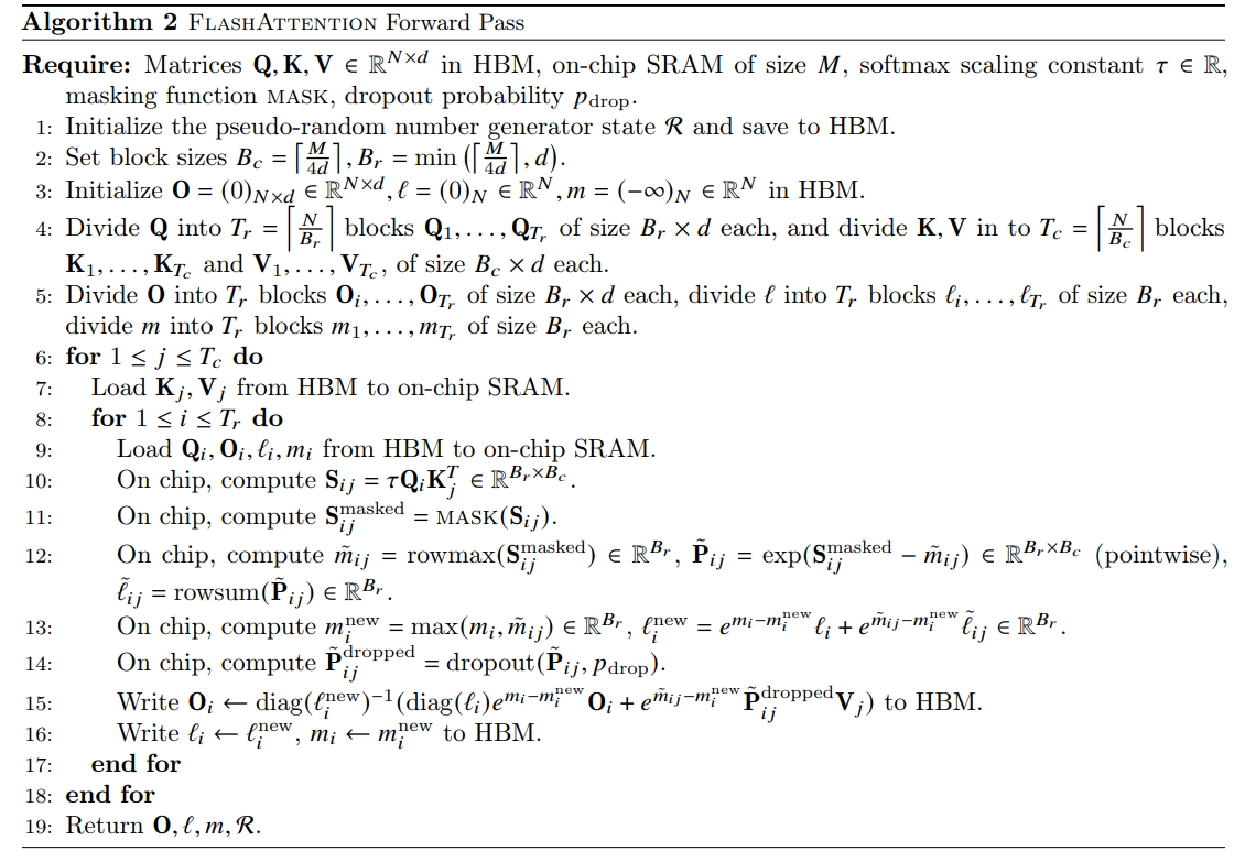
FlashAttention - Algorithm details
As one may understand, the materialization of the \(N \times N\) attention matrix on the HBM and its repeated reading and writing is a major bottleneck. To solve this, two main things need to be done -
- Computing the softmax reduction without access to the whole input
- Not storing the large intermediate attention matrix for the backward pass
Two established techniques, namely tiling and recomputation are used to solve this.
- Tiling - The attention computation is restructured to split the input into blocks and performing the softmax operation incrementally by making several passes over the input blocks.
- Recomputation - The softmax normalization factor from the forward pass is stored to quickly recompute attention on-chip in the backward pass, which is faster than the standard attention approach of reading the intermediate matrix from HBM.
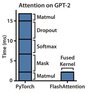
This does lead to increased FLOPs due to recomputation, however FlashAttention runs both faster (up to 7.6x on GPT-2) and uses less memory — linear in sequence length, due to the massively reduced amount of HBM access.
Understanding the algorithm
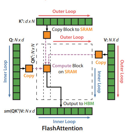
The main idea behind the algorithm is to split the inputs \(\mathbf{Q, K, V}\) into blocks, loading them from slow HBM to fast SRAM and then computing the attention output w.r.t those blocks. The output of each block is scaled by the right normalization factor before adding them up, which gives the correct result.
\[\mathbf{S} = \mathbf{\tau QK^\mathsf{T}} \in \mathbb{R}^{N \times N},\quad \mathbf{S}^\mathrm{masked} = \mathrm{MASK}(S) \in \mathbb{R}^{N \times N},\quad \mathbf{P} = softmax(\mathbf{S^\mathrm{masked}}) \in \mathbb{R}^{N \times N},\] \[\mathbf{P}^\mathrm{dropped} = \mathrm{dropout}(\mathbf{P}, p_\mathrm{drop}), \quad \mathbf{O} = \mathbf{P^\mathrm{dropped}V} \in \mathbb{R}^{N \times d},\]where \(\tau \in \mathbb{R}\) is some softmax scaling factor (typically \(\frac{1}{\sqrt{d}}\)), \(\mathrm{MASK}\) is some masking function that sets some entries of the input to \(-\infty\) and keep other entries the same, and \(\mathrm{dropout}(x, p)\) applies dropout to 𝑥 elementwise (i.e., output \(\frac{x}{1-p}\) with probability \(1 − p\) and output \(0\) with probability \(p\) for each element \(x\))
Tiling
The key part in understanding the block-wise computation of attention in the algorithm above is the block-wise computation of the softmax. The paper explains it well though. The softmax of a vector \(x \in \mathbb{R}^B\) can be computed as -

And for vectors \(x^\mathrm{(1)}, x^\mathrm{(2)} \in \mathbb{R}^B\), the softmax of the concatenated \(x = [x^\mathrm{(1)}, x^\mathrm{(2)}] \in \mathbb{R}^{2B}\) is given by -
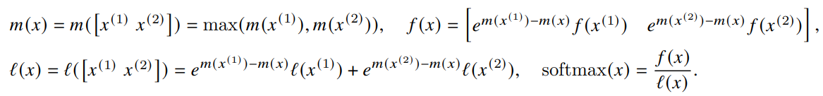
Let’s understand this better. In the above equations, \(m(x)\) holds the maximum between \(m(x^\mathrm{(1)})\) and \(m(x^\mathrm{(2)})\). Now, \(m(x^\mathrm{(1)})\) is the maximum element of \(x^\mathrm{(1)}\) and \(m(x^\mathrm{(2)})\) is the maximum element of \(x^\mathrm{(2)}\) which means that \(m(x)\) is basically the maximum of the whole concatenated vector. The beauty is that this was done blockwise.
So, if statistics \((m(x), l(x))\) are tracked then softmax can be computed one block at a time. In line 12 of the algorithm, \(\tilde{m_{ij}}\) has the maximum element of each row of \(S_{ij}^\mathrm{masked}\), and next in line 13, \(m_i^\mathrm{new}\) holds the row-wise maximum of the \(m_i\) till now and the new one i.e., \(\tilde{m_{ij}}\). Hence \(m_i\) is updated every column from the outer loop and eventually stores the row-wise max of the matrix \(\mathbf{S}\). The same logic goes for \(l_i\) and the matrix \(\mathbf{P}\). The results are combined to get the output attention matrix in line 15.
Recomputation
The backward pass of FlashAttention requires the \(\mathbf{S}\) and \(\mathbf{P}\) matrices to compute the gradients w.r.t \(\mathbf{Q}\), \(\mathbf{K}\), \(\mathbf{V}\). However, they are \(N \times N\) matrices and as it can be seen in the algorithm above, they aren’t stored explicitly. The trick is to use the output \(\mathbf{O}\) and the softmax normalization statistics \((m, l)\), we can recompute the attention matrix \(\mathbf{S}\) and \(\mathbf{P}\) easily in the backward pass from blocks of \(\mathbf{Q}\), \(\mathbf{K}\), \(\mathbf{V}\) in SRAM. even with more FLOPs, the recomputation step speeds up the backward pass due to reduced HBM accesses. The backward pass is very interesting too but slightly more complicated hence I’ll probably cover it in a separate post. One can cover the Appendix B of the paper to learn more.
Kernel Fusion is also used to implement the algorithm in one CUDA kernel, loading input from HBM, performing all the computation steps (matrix multiply, softmax, optionally masking and dropout, matrix multiply), then writing the result back to HBM. This avoids repeatedly reading and writing of inputs and outputs from and to HBM.
Important Information - The FlashAttention algorithm computed \(\mathbf{O} = softmax(QK^\mathsf{T})V\) with \(O(N^2d)\) FLOPs and requires \(O(N)\) additional memory beyond inputs and output (for the \((l, m)\) statistics).
The proof for the FLOPs calculation is given in Appendix C of the paper, which should be checked out by the curious reader.
Important Information - Let \(N\) be the sequence length, \(d\) be the head dimension, and \(M\) be the size of SRAM with \(d \leq M \leq Nd\). Standard attention requires \(\Theta(Nd + N^2)\) HBM accesses while FlashAttention requires \(\Theta(N^2d^2M^{-1})\) HBM accesses.
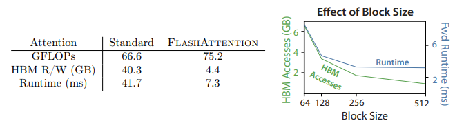
For typical values of \(d\) (64-128) and \(M\) (around 100KB), \(d^2\) is many times smaller than \(M\), and thus FlashAttention requires many times fewer HBM accesses than standard implementation. This leads to both faster execution and a lower memory footprint.
The authors also go on to show that the number of HBM accesses by FlashAttention is a lower-bound. There can be no implementation which can asymptotically improve on the number of HBM accesses for all values of \(M\) when doing exact attention calculation.
As the block size increases, the number of HBM accesses decreases as there are less passes over the input, and the runtime also decreases. However, beyond 256, the runtime starts getting bottlenecked by factors like arithmetic operations. And there is also a limit on how large we can choose the block size to be, as we want it to be able to fit in the SRAM.
Block-Sparse FlashAttention
As mentioned in the overview, FlashAttention can be used to make a approximate attention algorithm as well. The authors call it Block-Sparse FlashAttention and it is the fastest approximate attention algorithm. The memory complexity is smaller than FlashAttention by a factor proportional to the sparsity.
For inputs \(\mathbf{Q, K, V} \in \mathbb{R}^{N \times d}\) and a mask \(\tilde{\mathbf{M}} \in \{ 0,1 \}^{N \times N}\), we want to calculate -
\[\mathbf{S} = \mathbf{QK^\mathsf{T}} \in \mathbb{R}^{N \times N},\quad \mathbf{P} = softmax(\mathbf{S} \odot \mathbb{1}_{\tilde{\mathbf{\mathrm{M}}}}) \in \mathbb{R}^{N \times N},\quad \mathbf{O} = \mathbf{PV} \in \mathbb{R}^{N \times d}\]Given a pre-defined block sparsity mask \(\mathbf{M} \in \{ 0,1 \}^{N/B_r \times N/B_c}\), Algorithm 2 above can be adapted to only compute the nonzero blocks of the attention matrix. We can just skip the zero blocks. The Algorithm shown below describes the forward pass of Block-sparse FlashAttention.
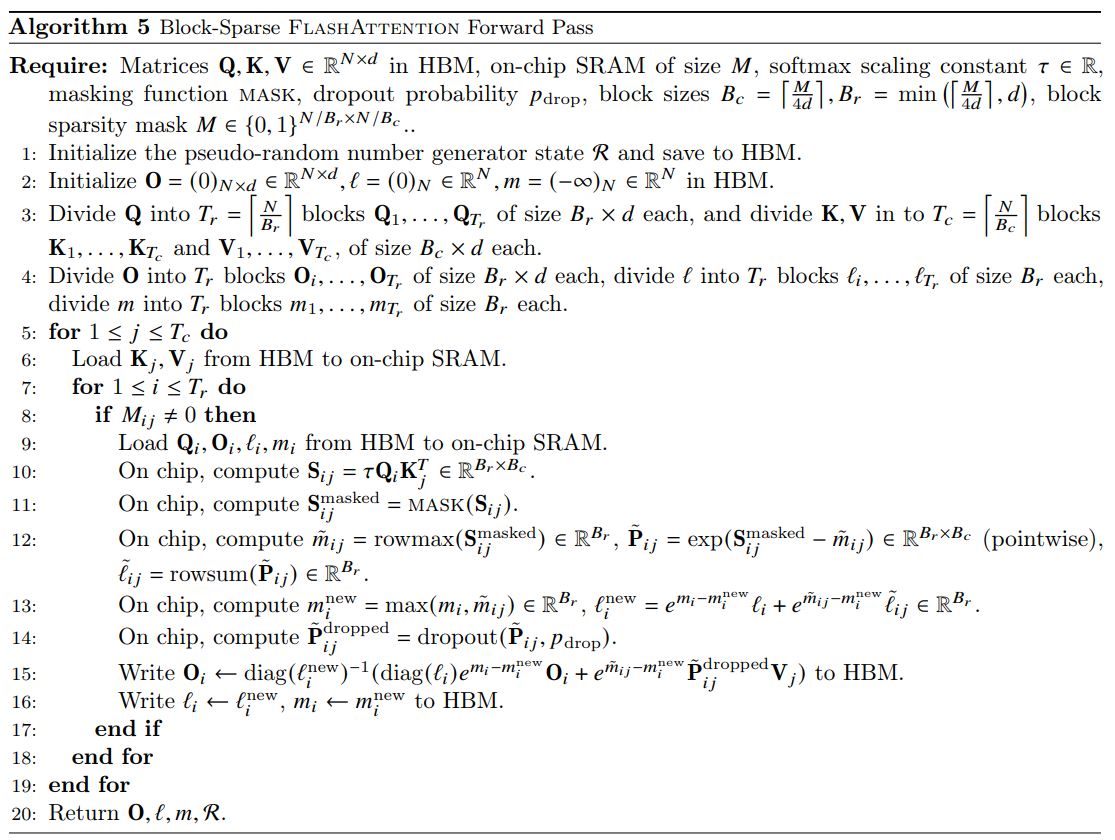
Important Information - Let \(N\) be the sequence length, \(d\) be the head dimension, and \(M\) be the size of SRAM with \(d \leq M \leq Nd\). Block-sparse FlashAttention requires \(\Theta(Nd + N^2d^2M^{-1}s)\) HBM accesses where \(s\) is the fraction of nonzero blocks in the block-sparsity mask.
For large sequence lengths, \(s\) is set to \(N^{-1/2}\) or \(N^{-1} \log N\) resulting in \(\Theta(N \sqrt{N})\) or \(\Theta(N \log N)\) IO complexity. As the sparsity increases, the runtime of block-sparse FlashAttention improves proportionally.
Experiments
There are tons of results in the paper. But the TL;DR is that FlashAttention beats all other exact attention algorithms in both training speed and quality of the models/down stream models especially when pushed to the limits of sequence length. I’ll add the plots and graphs for their various results here. Additional results are present in the paper.
Training Speed
BERT
GPT-2
Long-range Arena
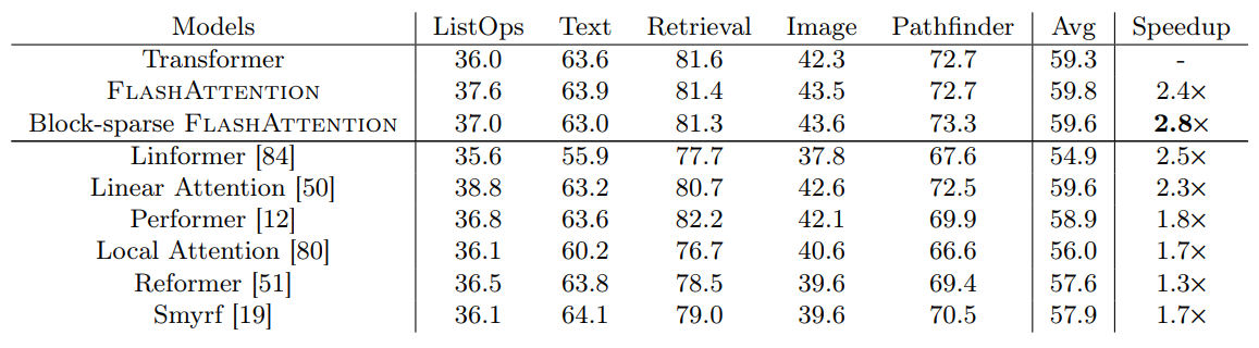
Block-sparse FlashAttention is faster than all of the approximate attention methods that were tested.
Model Quality
Language Modeling with Long Context
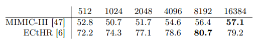
Long Document Classification
Since FlashAttention allows training on longer sequences, it improves performance on such datasets. MIMIC-III contains intensive care unit patient discharge summaries, each annotated with multiple labels. ECtHR contains legal cases from the European Court of Human Rights, each of which is mapped to articles of the Convention of Human Rights that were allegedly violated. Both of these datasets contain very long text documents. The average number of tokens in MIMIC-III is 2395 tokens and the longest document contains 14562 tokens.
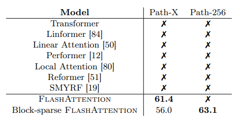
Path-X and Path-256
These are challenging tasks from the long range arena benchmark where the task is to classify whether two points in a black and white 128×128 (or 256×256) image have a path connecting them, and the images are fed to the transformer one pixel at a time. No transformer model in the past has been able to model these tasks effectively. They have either ran out of memory or achieved random performance. FlashAttention yields the first Transformer that can achieve better-than-random performance on the challenging Path-X task (sequence length 16K), and block-sparse FlashAttention yields the first sequence model that can achieve better-than-random performance on Path-256 (sequence length 64K).
Benchmarking Attention
Runtime
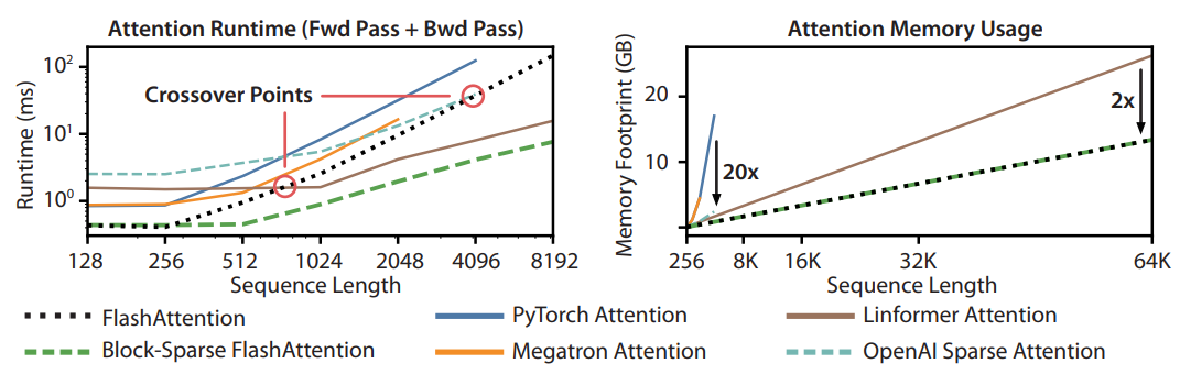
FlashAttention beats all exact attention baselines and is about 3× faster than the PyTorch implementation. The runtimes of many approximate/sparse attention mechanisms grow linearly with sequence length, but FlashAttention still runs faster than approximate and sparse attention for short sequences due to fewer memory accesses. The approximate attention runtimes begin to cross over with FlashAttention at sequences between 512 and 1024. On the other hand, block-sparse FlashAttention is faster than all implementations of exact, sparse, and approximate attention that are available, across all sequence lengths.
Memory Footprint
FlashAttention and block-sparse FlashAttention have the same memory footprint, which grows linearly with sequence length. FlashAttention is up to 20× more memory efficient than exact attention baselines, and is more memory-efficient than the approximate attention baselines. All other algorithms except for Linformer run out of memory on an A100 GPU before 64K, and FlashAttention is still 2× more efficient than Linformer.
A great paper overall, tremendous impact and personally, I had loads to learn from it!